Using VLOOKUP to Compare Two Lists in Excel: A Comprehensive Guide

Comparing two lists in Excel can be a time-consuming and error-prone task if done manually. Whether you’re reconciling financial records, managing inventory, or updating customer databases, accurately identifying discrepancies is crucial. Fortunately, Excel’s VLOOKUP function offers a powerful and efficient way to compare two lists and pinpoint the differences. This guide will walk you through a step-by-step process to use VLOOKUP to compare lists, making data reconciliation faster and more accurate.

Understanding VLOOKUP for List Comparison

VLOOKUP, short for “Vertical Lookup,” is an Excel function designed to search for a value in the first column of a table and return a corresponding value from another column in the same row. While primarily used for data retrieval, VLOOKUP’s ability to check for the existence (or absence) of a value in a table makes it exceptionally useful for comparing lists.

When comparing two lists, VLOOKUP can help you answer questions like:

Which items from List A are also present in List B?
Which items from List A are missing from List B?
Are there any discrepancies between the two lists?

This technique is invaluable in various scenarios, such as:

Financial Reconciliation: Accountants can compare their invoice records against client records to identify missing invoices.
Inventory Management: Businesses can compare their inventory lists with sales records to track stock levels and identify discrepancies.
Data Cleansing: Analysts can compare datasets to find duplicate entries or inconsistencies.
HR Management: HR departments can compare employee lists against payroll data to ensure accurate records.

To effectively use VLOOKUP for list comparison, it’s important to understand its core mechanics and how to adapt it for this specific purpose.

Step-by-Step Guide to Comparing Lists with VLOOKUP

Let’s break down the process of comparing two lists using VLOOKUP in Excel. We will use the example of comparing an “Invoice Report” with a “Customer Report” to identify missing invoices in the customer’s record.

1. Prepare Your Data and Identify a Unique Lookup Value

Before you start building your VLOOKUP formula, ensure your data is properly organized. For VLOOKUP to work effectively, you need:

Two Lists: These are the lists you want to compare. In our example, these are the “Invoice Report” and the “Customer Report.”
A Common Identifier (Lookup Value): There must be at least one column that is common to both lists and can uniquely identify each record. In our example, the “Invoice Number” is the ideal lookup value as it should be unique for each invoice. While Date or Amount could be used, Invoice Number is less likely to have duplicates and is therefore more reliable.

It’s a best practice to check for duplicate values in your chosen lookup column within each list to ensure accuracy. Select the column, go to Home > Conditional Formatting > Highlight Cells Rules > Duplicate Values to quickly identify and address any duplicates.

Also, remember that VLOOKUP searches from left to right. The lookup value column must be the first column in the table array you will define in the VLOOKUP formula.

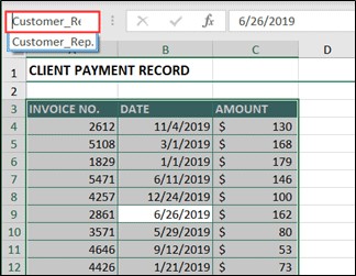
2. Name Ranges for Formula Efficiency (Optional but Recommended)

Naming your data ranges makes your formulas easier to read, understand, and maintain. It also simplifies the process of creating VLOOKUP formulas.

Go to the worksheet containing your second list (in our example, the ‘Customer Report‘ worksheet).
Select all the data in the list, including headers if you wish to include them in your named range (Click on a cell within the data and press Ctrl+A or Cmd+A on Mac).
In the Name Box (located to the left of the formula bar), type a descriptive name for this range, like Customer_Report_Data. Avoid spaces in range names; use underscores instead.
Press Enter.

3. Construct the Basic VLOOKUP Formula to Compare Lists

Now, let’s build the VLOOKUP formula in the first list (the ‘Invoice Report‘ worksheet) to compare it against the ‘Customer Report‘ list.

Go to the ‘Invoice Report‘ worksheet and select the first empty column next to your data (e.g., column E). In the first data row (e.g., cell E4), enter the VLOOKUP formula:
```
=VLOOKUP(A4,Customer_Report_Data,1,FALSE)
```
Let’s break down this formula:
- =VLOOKUP(: Starts the VLOOKUP function.
- A4: This is the lookup_value. It’s the Invoice Number from the current row in the ‘Invoice Report‘ (cell A4). Excel will look for this invoice number in the ‘Customer_Report_Data‘ range.
- Customer_Report_Data: This is the table_array. It’s the named range we created earlier, representing the ‘Customer Report‘ data. VLOOKUP will search for the lookup value in the first column of this range (which should be the Invoice Number column in your ‘Customer Report‘).
- 1: This is the col_index_num. It specifies which column to return a value from if a match is found. In this case, we use 1 because we simply want to confirm if the Invoice Number exists in the second list. We can return a value from the first column itself (Invoice Number) as confirmation.
- FALSE: This is the range_lookup. FALSE (or 0) specifies that we want an exact match for the lookup value. This is crucial for accurate list comparison.
Press Enter. The cell E4 will now display either an Invoice Number (if a match is found in the ‘Customer Report‘) or #N/A (if the Invoice Number is not found).
Use the fill handle (the small square at the bottom-right of the selected cell) to drag the formula down to apply it to all rows in your ‘Invoice Report‘ list.

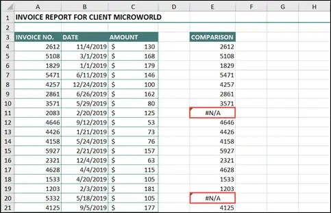
4. Understand and Interpret #N/A Errors

The #N/A error is Excel’s way of saying “Value Not Available.” In the context of VLOOKUP for list comparison, a #N/A error in column E next to an invoice in the ‘Invoice Report‘ indicates that this specific invoice number is missing from the ‘Customer Report‘ list. Conversely, if you see an invoice number displayed, it means that invoice exists in both lists.

![VLOOKUP results showing #N/A errors for missing records](http://compare.edu.vn/wp-content/uploads/2025/02/image-10.jpg){width=483 height=311}
*Alt text: VLOOKUP results in Excel column E showing invoice numbers for matches and #N/A errors for missing invoices in the compared list.*

5. Improve Readability with ISNA and IF Functions

While #N/A errors are informative, they might not be the most user-friendly way to present the comparison results. We can enhance the report’s clarity by using the ISNA and IF functions to display more meaningful text instead of #N/A.

Wrap VLOOKUP with ISNA: In cell E4, modify the formula to include the ISNA function:
```
=ISNA(VLOOKUP(A4,Customer_Report_Data,1,FALSE))
```
The ISNA function checks if a value is #N/A. It returns TRUE if the VLOOKUP results in #N/A (meaning the invoice is missing) and FALSE otherwise.
Press Enter and use the fill handle to copy the formula down. Now, column E will display TRUE for missing invoices and FALSE for matching invoices.
Use IF for Meaningful Output: To display more descriptive text, wrap the ISNA formula with an IF function:
```
=IF(ISNA(VLOOKUP(A4,Customer_Report_Data,1,FALSE)),"Missing Record","")
```
The IF function has three parts:
- logical_test: ISNA(VLOOKUP(A4,Customer_Report_Data,1,FALSE)) – This is our ISNA formula, which returns TRUE if the record is missing.
- value_if_true: "Missing Record" – If the ISNA function returns TRUE (record is missing), the formula will display “Missing Record”.
- value_if_false: "" – If the ISNA function returns FALSE (record is found), the formula will display nothing (an empty string). You can replace "" with "Record Found" or any other text if you prefer.
Press Enter and use the fill handle to copy the formula down. Column E now clearly indicates “Missing Record” for invoices not found in the ‘Customer Report‘ and leaves the cell blank for invoices that are present in both lists.

6. Highlight Missing Records with Conditional Formatting (Advanced)

For a visually impactful report, use conditional formatting to automatically highlight entire rows of missing records.

Select the data range in your ‘Invoice Report‘ that you want to highlight (e.g., A4:C50).
Go to the Home tab on the Excel ribbon and click on Conditional Formatting.
Select New Rule.
In the ‘New Formatting Rule’ dialog box, choose “Use a formula to determine which cells to format”.
In the “Format values where this formula is true” box, enter the following formula:
```
=ISNA(VLOOKUP($A4,Customer_Report_Data,1,FALSE))
```
Important: Note the $ before A4 in $A4. This is crucial. It makes the column reference absolute (always column A), while the row reference remains relative (changes as conditional formatting is applied to each row). This ensures the formula checks the Invoice Number in column A for each row.
Click the Format button to choose how you want to highlight the missing records (e.g., fill color, font style).
Click OK twice to apply the conditional formatting.

Now, all rows in your ‘Invoice Report‘ where the Invoice Number is not found in the ‘Customer Report‘ will be automatically highlighted, making it very easy to visually identify the missing records.

Best Practices and Considerations

Ensure Data Integrity: Before comparing lists, double-check for data consistency, especially in the lookup value column. Inconsistent formatting (e.g., spaces, different case) can lead to VLOOKUP failing to find matches.
Choose the Right Lookup Value: Select a lookup value that is unique and reliably present in both lists.
Optimize for Large Datasets: For very large lists, consider using Excel Tables and structured references for better performance and formula management.
Explore Alternatives: While VLOOKUP is effective, Excel also offers other functions for list comparison, such as MATCH, COUNTIF, and Power Query, which might be more suitable for specific scenarios or complex comparisons.

By mastering VLOOKUP for list comparison, you can significantly enhance your data analysis capabilities in Excel, saving time and improving accuracy in various data reconciliation tasks.