Quick Excel Column Comparison: Spot Identical Matches Instantly

Data analysis often requires comparing columns to identify similarities or differences. Manually checking each cell can be incredibly time-consuming, especially with large datasets. Fortunately, Excel offers several efficient methods to compare columns in seconds. If you’re looking for a Short Formula To Compare Two Columns In Excel If Same, you’ve come to the right place.

Understanding Column Comparison in Excel

Comparing columns in Excel simply means checking corresponding cells in two or more columns to see if they match. This can be used to find duplicate entries, identify unique values, or highlight discrepancies between datasets.

Let’s explore some practical methods to achieve this efficiently.

Simple Methods to Compare Two Columns in Excel

Here are several straightforward techniques to compare columns in Excel, starting with the quickest formulas:

• Equals Operator (=)
• IF Formula
• Conditional Formatting
• VLOOKUP Function
• EXACT Formula

Using the Equals Operator: A Quick Check

The equals operator is the most basic and fastest way to compare two columns in Excel for exact matches.

Steps:

1. Create a Result Column: Insert a new column next to the columns you want to compare.

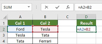
2. Enter the Formula: In the first cell of the result column (e.g., cell C2 if you are comparing A and B starting from row 2), type the formula =A2=B2.

3. Apply to All Cells: Drag the fill handle (the small square at the bottom right of the cell) down to apply the formula to all rows you need to compare.

Result:

Excel will display TRUE if the values in the corresponding cells of the two columns are identical, and FALSE otherwise.

Customizing the Output with IF Formula

For a more user-friendly output than TRUE or FALSE, you can combine the equals operator with the IF formula. This allows you to display custom messages like “Match” or “No Match”.

Formula: =IF(A2=B2, "Match", "No Match")

Steps:

1. Enter the Modified Formula: In the result column, use the formula =IF(A2=B2, "Match", "No Match").

2. Apply to All Cells: Drag the fill handle down to apply the formula to the rest of the rows.

Result:

Now, the result column will show “Match” when the values in the compared cells are the same, and “No Match” when they are different.

Conditional Formatting: Visually Highlight Matches or Differences

Conditional formatting offers a visual way to compare columns by highlighting matching or unique values directly within the columns.

Steps:

1. Select Columns: Select the two columns you want to compare.

2. Conditional Formatting: Go to the “Home” tab on the Excel ribbon, click on “Conditional Formatting” in the “Styles” group.

3. Highlight Cells Rules: Choose “Highlight Cells Rules” and then select “Duplicate Values” or “Unique Values” depending on what you want to highlight.

4. Choose Duplicate or Unique: In the “Duplicate Values” dialog box, select either “Duplicate” to highlight matching entries or “Unique” to highlight different entries. Choose your desired formatting style (e.g., fill color, font color).

5. Click OK: Excel will instantly highlight the duplicate or unique values based on your selection within the chosen columns.

VLOOKUP Function: Checking for Presence and Extracting Data

The VLOOKUP function is more versatile and can be used to compare columns by checking if values from one column exist in another and even retrieve corresponding data.

Formula: =VLOOKUP(lookup_value, table_array, col_index_num, [range_lookup])

To compare two columns and identify matches from Column A in Column B:

Steps:

1. Create a Result Column: Add a new column for results.

2. Enter VLOOKUP Formula: In the first cell of the result column, enter the formula =VLOOKUP(A2, B:B, 1, FALSE). Here, A2 is the value you are looking up from column A, B:B is the column you are searching in (Column B), 1 means return the value from the first column of the table_array (which is Column B itself in this case), and FALSE ensures an exact match.

3. Apply to All Cells: Drag the fill handle down.

Result:

• If a value from Column A is found in Column B, VLOOKUP will return that value.

• If a value from Column A is not found in Column B, VLOOKUP will return a #N/A error.

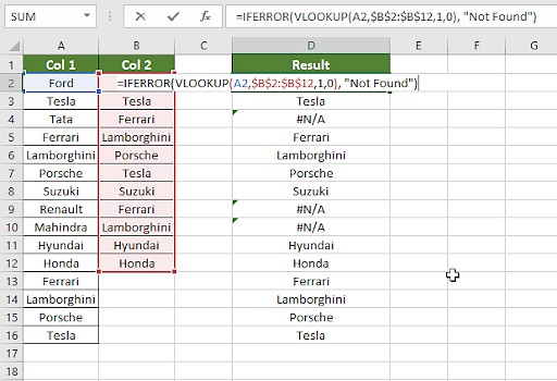
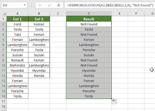
Handling Errors with IFERROR

To replace the #N/A errors with more descriptive messages, use the IFERROR function:

Modified Formula: =IFERROR(VLOOKUP(A2, B:B, 1, FALSE), "Not Found in Column B")

![Compare_columns_in_Excel_12.](http://compare.edu.vn/wp-content/uploads/2025/02/comparecolumnsinexcel12.jpg){width=512 height=350}

Result:

Now, instead of errors, you’ll see “Not Found in Column B” for values from Column A that are not present in Column B.

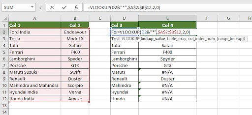
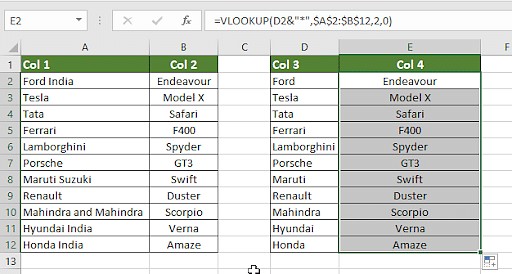
![Compare_columns_in_Excel_13.](http://compare.edu.vn/wp-content/uploads/2025/02/comparecolumnsinexcel13.jpg){width=512 height=367}

Dealing with Partial Matches using Wildcards in VLOOKUP

In scenarios where you need to compare columns with slight variations, like “Ford India” vs. “Ford”, you can use wildcards with VLOOKUP.

Example: To find “Ford” even if Column B has “Ford India”, you can modify the lookup value:

Formula with Wildcard: =IFERROR(VLOOKUP(A2&"*", B:B, 1, FALSE), "Not Found")

![Compare_columns_in_Excel_15](http://compare.edu.vn/wp-content/uploads/2025/02/comparecolumnsinexcel15.jpg){width=512 height=234}

Result:

This formula will now consider “Ford India” in Column B a match for “Ford” in Column A.

![Compare_columns_in_Excel_16.](http://compare.edu.vn/wp-content/uploads/2025/02/comparecolumnsinexcel16.jpg){width=512 height=274}

EXACT Formula: Case-Sensitive Comparison

The EXACT formula is used when you need a case-sensitive comparison. It distinguishes between “Apple” and “apple”.

Formula: =EXACT(A2, B2)

Steps:

1. Enter EXACT Formula: In a result column, type =EXACT(A2, B2).

2. Apply to All Cells: Drag the fill handle down.

Result:

EXACT returns TRUE only if the cell contents are exactly the same, including case, and FALSE otherwise.

Choosing the Right Method for Your Scenario

Here’s a quick guide to help you select the best method for different comparison needs:

Scenario 1: Row-by-Row Comparison for Matches

For basic row-by-row comparison to see if values in two columns match, use:

• =IF(A2=B2, "Match", " ") (Case-insensitive)
• =IF(EXACT(A2, B2), "Match", " ") (Case-sensitive)

Scenario 2: Comparing Multiple Columns

To check for matches across multiple columns in the same row:

• =IF(AND(A2=B2, A2=C2), "Complete Match", " ") (All columns must match)
• =IF(COUNTIF($A2:$E2, $A2)=4, "Complete Match", " ") (At least 4 out of 5 columns match the first column, adjust the number as needed)

Scenario 3: Finding Unique Values in One Column Compared to Another

To find values in Column A that are not present in Column B:

• =IF(COUNTIF($B:$B, $A2)=0, "Not in Column B", " ")
• =IFERROR(MATCH($A2,$B$2:$B$10,0),"Not in Column B","")

To find matches and unique values in one formula:

• =IF(COUNTIF($B:$B, $A2)=0, "Unique to Column A", "Present in Column B")

Scenario 4: Comparing Lists and Extracting Matches

To compare two lists and pull matching data from a second list based on matches in the first:

• =VLOOKUP(D2, $A$2:$B$6, 2, FALSE) (Finds value from Column D in Column A and returns corresponding value from Column B)
• =INDEX($B$2:$B$6, MATCH($D2, $A$2:$A$6, 0)) (Alternative to VLOOKUP, more flexible)
• =XLOOKUP(D2, $A$2:$A$6, $B$2:$B$6) (Modern replacement for VLOOKUP and INDEX/MATCH, simpler syntax)

Scenario 5: Highlighting Row Matches and Differences Visually

To visually highlight entire rows where columns match or differ, use Conditional Formatting with formulas:

• =AND($A2=$B2, $A2=$C2) (Highlight rows where Columns A, B, and C match)
• =COUNTIF($A2:$C2, $A2)=3 (Same as above, for 3 columns)

Alternatively, to quickly highlight row differences:

1. Select the dataset.

2. Go to “Home” tab -> “Find & Select” -> “Go To Special”.

3. Choose “Row Differences” and click “OK”.

4. Excel will select cells with different values in each row, which you can then format (e.g., change fill color).

FAQs on Comparing Columns in Excel

1. What is the quickest way to compare two columns in Excel?

The quickest way is to use the equals operator (=) in a new column, like =A2=B2, to get TRUE/FALSE results. For slightly more descriptive output, use =IF(A2=B2, "Match", "No Match").

2. Can I use INDEX-MATCH to compare columns?

Yes, INDEX-MATCH is a powerful alternative to VLOOKUP and can be used for column comparison, especially when you need more flexibility in lookups.

3. How do I compare multiple columns at once?

Use formulas like AND and COUNTIF within IF statements, or use Conditional Formatting with formulas to compare multiple columns for matches or differences.

4. How can I compare two lists for matches in Excel?

You can use VLOOKUP, MATCH, or XLOOKUP to compare lists and find matching entries. COUNTIF is also useful for checking if values from one list exist in another.

5. How do I highlight duplicates when comparing two columns?

Use Conditional Formatting:

1. Select the columns.
2. Go to “Home” -> “Conditional Formatting” -> “Highlight Cells Rules” -> “Duplicate Values”.
3. Choose your desired formatting and click “OK”.

Next Steps in Data Analysis with Excel

Now that you’ve mastered comparing columns, consider exploring Pivot Charts in Excel. They are essential for creating interactive dashboards and gaining deeper insights from your data.

To further enhance your data analysis skills, consider a comprehensive Data Analyst Master’s Program. This will equip you with advanced techniques and tools to excel in the field of data analytics. Start your learning journey today!