How to Compare Two Tabs in Excel: Simple to Advanced Techniques

When working with Microsoft Excel, you often find yourself managing large datasets spread across multiple worksheets, or “tabs”. Whether you’re tracking sales figures, managing project data, or analyzing survey results, the need to compare information between these tabs is a common and crucial task. Knowing How To Compare Two Tabs In Excel efficiently can save you significant time, reduce errors, and provide deeper insights into your data.

This comprehensive guide will explore various methods to compare two tabs in Excel, ranging from simple visual techniques to more advanced formulas, conditional formatting, and powerful third-party tools. We’ll delve into each approach, highlighting its strengths, limitations, and step-by-step instructions to empower you with the skills to effectively compare your Excel worksheets and identify the differences that matter most.

Visual Side-by-Side Comparison: A Quick Glance

For a preliminary overview, or when dealing with smaller datasets, the “View Side by Side” feature in Excel offers a straightforward way to visually compare two tabs. This method is ideal for quickly spotting obvious discrepancies and understanding the general layout differences between your worksheets.

Comparing Tabs in the Same Workbook Side by Side

If the two tabs you wish to compare are within the same Excel workbook, follow these steps to view them side by side:

Open your Excel workbook that contains the tabs you want to compare.
Navigate to the View tab on the Excel ribbon.
In the Window group, click on the New Window button. This action will open a new window displaying the same workbook.
In either of the two workbook windows, click the View Side by Side button, also located in the Window group of the View tab.
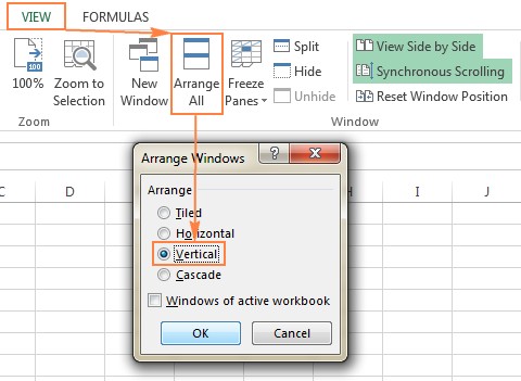
Excel will automatically arrange the two workbook windows horizontally by default. To switch to a vertical arrangement, click the Arrange All button (next to “View Side by Side”) and select Vertical.

Now, you’ll have two instances of your Excel workbook displayed side by side, allowing you to navigate to different tabs in each window. Select the first tab you want to compare in one window and the second tab in the other window. You can now scroll through both worksheets simultaneously for a visual comparison.

To ensure synchronized scrolling, check if the Synchronous Scrolling option is enabled. This feature is typically activated automatically when you use “View Side by Side” and is located directly beneath the “View Side by Side” button on the View tab.

Comparing Tabs from Different Workbooks Side by Side

The “View Side by Side” feature can also be used to compare tabs from two different Excel workbooks. The process is even simpler:

Open both Excel workbooks that contain the tabs you want to compare.
Ensure that both workbooks are active (i.e., one of their windows is currently selected).
Go to the View tab in either workbook.
Click the View Side by Side button in the Window group.
If Excel doesn’t automatically arrange the specific workbooks you want to compare, a Compare Side by Side dialog box may appear. In this dialog, select the workbook you want to display alongside the currently active workbook.

Excel will then arrange the selected workbooks side by side, enabling you to choose the specific tabs you want to compare within each workbook window.

Formula-Based Comparison: Identifying Value Differences

For a more precise comparison, especially when you need to pinpoint exact value differences between two tabs, Excel formulas provide a powerful solution. By using a simple IF formula, you can generate a difference report directly within a new worksheet.

Creating a Difference Report with Formulas

Here’s how to set up a formula to compare two tabs and highlight value discrepancies:

Open your Excel workbook containing the two tabs you want to compare (e.g., “Sheet1” and “Sheet2”).
Insert a new blank worksheet where you will create the difference report.
In cell A1 of the new sheet, enter the following formula:
```
=IF(Sheet1!A1<>Sheet2!A1, "Sheet1:"&Sheet1!A1&" vs Sheet2:"&Sheet2!A1, "")
```
Explanation of the formula:
- Sheet1!A1<>Sheet2!A1: This part compares the value in cell A1 of “Sheet1” with the value in cell A1 of “Sheet2”. The <> operator means “not equal to”.
- "Sheet1:"&Sheet1!A1&" vs Sheet2:"&Sheet2!A1: If the values are different, this part constructs a text string indicating the values from both sheets.
- "": If the values are the same, this part returns an empty string, leaving the cell blank in the difference report.
Copy the formula down and to the right to cover the entire range of data you want to compare in both tabs. You can easily do this by selecting cell A1, then dragging the fill handle (the small square at the bottom-right corner of the selected cell) across the rows and columns.

The new worksheet will now display a difference report. Cells will remain blank if the corresponding cells in “Sheet1” and “Sheet2” have identical values. If there are differences, the cells in the report will show a text string detailing the values from both sheets, clearly indicating the discrepancies.

Limitations of Formula-Based Comparison:

Value Comparison Only: This method only compares cell values. It does not identify differences in formulas or cell formatting.
Row/Column Sensitivity: If rows or columns have been added or deleted in one tab compared to the other, the comparison will become misaligned from the point of insertion/deletion onwards.
Date Representation: Dates might be represented as serial numbers in the difference report, which can be less intuitive for analysis.

Conditional Formatting: Visually Highlighting Differences

Conditional formatting offers a visually appealing and dynamic way to highlight cells with different values directly within one of your tabs. This method is excellent for quickly spotting discrepancies within the data itself, without creating a separate report.

Highlighting Differences with Conditional Formatting Rules

Follow these steps to use conditional formatting to highlight cells that differ between two tabs:

Select the data range in the worksheet where you want to highlight the differences. Typically, you’ll want to select the entire used range of your data. Start by clicking the top-left cell of your data range (usually A1) and press Ctrl + Shift + End to extend the selection to the last used cell.
Go to the Home tab on the Excel ribbon.
In the Styles group, click on Conditional Formatting and then select New Rule.
In the New Formatting Rule dialog box, choose the rule type “Use a formula to determine which cells to format”.
In the “Format values where this formula is true” box, enter the following formula:
```
=A1<>Sheet2!A1
```
Replace “Sheet2” with the actual name of the other tab you are comparing. A1 in this formula refers to the top-left cell of your selected range in step 1. Excel will automatically adjust this relative reference for all other cells in your selection.
Click the Format button to choose the formatting style for cells with differences. You can change the fill color, font style, border, etc.
Click OK in both the Format Cells and New Formatting Rule dialog boxes.

Excel will now apply the conditional formatting rule to your selected range. Any cell in the first tab that has a different value compared to the corresponding cell in “Sheet2” will be highlighted with the formatting style you selected, making it easy to visually identify the differences.

Limitations of Conditional Formatting Comparison:

Value Comparison Only: Similar to formula-based comparison, conditional formatting only focuses on value differences and ignores formula or formatting discrepancies.
Row/Column Sensitivity: Added or deleted rows/columns will cause misalignment in the comparison.
One-Way Highlighting: Differences are highlighted only in the worksheet where you apply the conditional formatting. You won’t see highlights in the second tab.

Advanced Comparison with “Compare and Merge Workbooks” (For Older Excel Versions)

For users of older versions of Excel (Excel 2010 through Excel 365), the “Compare and Merge Workbooks” feature offers a way to track and merge changes made by multiple users in shared workbooks. While primarily designed for collaborative scenarios, it can also be adapted for comparing different versions of the same workbook or, indirectly, different tabs if they were saved as separate workbooks.

Note: This feature is less prominent in newer Excel versions and might be replaced by more modern collaboration tools like co-authoring in Microsoft 365.

Enabling and Using “Compare and Merge Workbooks”

Add the command to the Quick Access Toolbar: By default, “Compare and Merge Workbooks” is not readily accessible. To add it, click the File tab, then Options, and select Quick Access Toolbar. In the “Choose commands from” dropdown, select All Commands. Scroll down to find “Compare and Merge Workbooks”, select it, click Add, and then OK. The command will appear in your Quick Access Toolbar (the small icons at the very top left of your Excel window).
Prepare your workbooks: To use this feature effectively, you ideally should have started with a shared workbook and had different users save copies with unique filenames as they made edits. To “share” a workbook (for the purpose of enabling change tracking), go to the Review tab, Changes group, and click Share Workbook (Legacy). Check the box “Allow changes by more than one user at the same time…” and click OK. Save the workbook.
Merge workbooks: Open the original “shared” workbook. Click the Compare and Merge Workbooks command in your Quick Access Toolbar. In the dialog box, select the copies of the workbook that you want to merge into the original. Hold the Shift key to select multiple files. Click OK.
Review changes: Excel will merge the changes from the selected copies into the original workbook. To visualize the changes, go to the Review tab, Changes group, and click Track Changes > Highlight Changes. In the “Highlight Changes” dialog, configure the settings (e.g., “When: All”, “Who: Everyone”, check “Highlight changes on screen”) and click OK.

Excel will highlight cells that have been changed, indicating who made the change and when. This can help you understand the differences between the merged versions, which can indirectly help compare different states of tabs if you saved them as separate workbooks.

Limitations of “Compare and Merge Workbooks”:

Legacy Feature: This feature is older and less suited for modern collaboration workflows.
Shared Workbook Requirement: It’s designed for merging changes in “shared workbooks,” which might require some setup.
Indirect Tab Comparison: You are not directly comparing tabs but rather merging changes from different file versions, which can be less direct for simply comparing two tabs.

Specialized Third-Party Tools: Comprehensive Excel Comparison

For users who frequently need to compare Excel files and tabs, and require more advanced features and accuracy, numerous third-party tools are available. These tools often go beyond the limitations of built-in Excel features, offering comprehensive comparison of values, formulas, formatting, and even structural differences like added or deleted rows and columns.

Here’s an overview of some popular third-party Excel comparison tools:

1. Synkronizer Excel Compare

Synkronizer Excel Compare is a powerful add-in that provides a wide range of comparison and merging capabilities. Key features include:

Comprehensive Comparison: Compares values, formulas, cell formats, comments, and names.
Difference Highlighting: Highlights differences directly in the worksheets with different colors for various types of changes.
Detailed Reports: Generates summary and detailed reports of differences, including hyperlinked reports for easy navigation.
Merge and Update: Allows you to merge changes selectively from one sheet to another, updating your primary worksheet.
Sheet and Workbook Comparison: Compares entire workbooks and individual worksheets.
Comparison Options: Offers various comparison modes like “normal worksheets,” “with link options,” “as database,” and range comparison.
Filtering: Allows filtering of differences to focus on specific types of changes (e.g., ignore case, spaces, formula differences).

2. Ablebits Compare Sheets for Excel (Part of Ultimate Suite)

Ablebits Compare Sheets is another robust tool, integrated within their Ultimate Suite for Excel add-in. It focuses on user-friendliness and intuitive workflow:

Step-by-Step Wizard: Guides you through the comparison process with a clear wizard interface.
Comparison Algorithms: Offers different algorithms (No key columns, By key columns, Cell-by-cell) to suit various data structures.
Review Differences Mode: Opens compared sheets side-by-side in a special “Review Differences” mode, allowing you to examine differences one by one and decide to merge or ignore them.
Backup Creation: Automatically creates backup copies of your workbooks before comparison.
Highlighting and Merging: Visually highlights differences and provides tools for merging changes between sheets.
Format Comparison: Can compare cell formatting as well as values and formulas.

3. xlCompare

xlCompare is a dedicated Excel comparison utility with a strong focus on accuracy and merging capabilities:

Workbook, Sheet, and VBA Comparison: Compares workbooks, worksheets, named ranges, and VBA projects.
Difference Identification: Detects added, deleted, and changed data.
Merge Differences: Provides tools for quickly merging differences between files.
Duplicate Finding and Removal: Can find and remove duplicate records between sheets.
Data Update and Merge: Allows updating records, adding unique rows/columns, and merging updated records between sheets.
Filtering and Highlighting: Offers filtering of comparison results and color-coded highlighting of differences.

4. Change Pro for Excel

Change Pro for Excel is designed for both desktop and mobile Excel comparison, with a focus on identifying a broad range of changes:

Formula, Value, and Layout Comparison: Compares formulas, values, and layout changes (rows/columns).
Embedded Object Recognition: Recognizes differences in charts, graphs, and images.
Difference Reports: Creates detailed reports of formula, value, and layout differences.
Filtering and Sorting: Allows filtering and sorting of difference reports.
Integration: Can compare files directly from Outlook and document management systems.
Multi-language Support: Supports all languages, including multi-byte character sets.

Online Excel Comparison Services: Quick and Easy

For occasional comparisons or when you need a quick solution without installing software, several online services offer Excel file and sheet comparison. These services typically involve uploading your Excel files to their website for comparison.

Caution: Be mindful of security when using online services, especially if your Excel files contain sensitive or confidential information.

Examples of online Excel comparison services include:

XLComparator (https://www.xlcomparator.net/): A free online tool for comparing Excel files.
CloudyExcel: Another online service that highlights differences between Excel sheets directly in the browser.

These online services are generally very easy to use. You typically upload your two Excel workbooks, and the service will process them and display the differences, often highlighting them directly in the sheets within your browser.

Choosing the Right Method

The best method for comparing two tabs in Excel depends on your specific needs and the complexity of your data:

Visual Side-by-Side Comparison: Ideal for quick, high-level comparisons and smaller datasets. Simple and built-in.
Formula-Based Comparison: Good for identifying value differences and creating basic difference reports. Built-in and requires some formula knowledge.
Conditional Formatting: Excellent for visually highlighting differences directly within a worksheet. Built-in and dynamic.
“Compare and Merge Workbooks” (Legacy): Useful for merging changes in older “shared workbook” scenarios, but less relevant for modern workflows. Built-in (older versions).
Third-Party Tools (e.g., Synkronizer, Ablebits, xlCompare): Best for comprehensive, accurate comparisons, especially when you need to compare formulas, formatting, and structural changes, and require merging capabilities. Add-ins or separate software, often paid.
Online Services (e.g., XLComparator, CloudyExcel): Convenient for quick, occasional comparisons without software installation. Web-based, consider security for sensitive data.

By understanding these different techniques for how to compare two tabs in Excel, you can choose the most effective method to analyze your data, identify discrepancies, and ensure data accuracy and consistency across your spreadsheets. Whether you opt for the simplicity of visual comparison, the precision of formulas, or the power of specialized tools, Excel provides a range of options to meet your comparison needs.