How To Compare Values In Excel And Highlight Differences?

Are you looking for How To Compare Values In Excel And Highlight Differences to streamline your data analysis? COMPARE.EDU.VN provides you with detailed methods and tools to effectively compare data in Excel, identify matches and differences, and visually highlight them for better insights. Discover the best strategies to enhance your data comparison skills and make informed decisions, boosting efficiency and accuracy in your data handling tasks. Explore this guide for expert tips and techniques.

1. Understanding the Basics of Value Comparison in Excel

Excel is a powerful tool for data analysis, and one of its fundamental capabilities is comparing values. Comparing values in Excel allows you to identify similarities and differences, which is crucial for various tasks such as data validation, reconciliation, and identifying trends. Whether you’re comparing two columns of data or multiple datasets, Excel offers several methods to achieve your goals.

1.1. Why Compare Values in Excel?

Comparing values in Excel is essential for a multitude of reasons:

Data Validation: Ensure that data entries are consistent and accurate.
Reconciliation: Identify discrepancies between two sets of data, such as financial records.
Trend Analysis: Spot patterns and anomalies in datasets over time.
Decision Making: Provide a clear basis for making informed decisions based on data.
Reporting: Create reports that highlight key differences and similarities.

1.2. Basic Techniques for Value Comparison

Before diving into advanced methods, it’s important to understand the basic techniques for comparing values in Excel. These techniques include using formulas, conditional formatting, and built-in functions.

Formulas: Simple formulas like =A1=B1 can quickly check if two cells have the same value.
Conditional Formatting: Highlight cells based on whether they meet certain criteria, such as being different from another cell.
Built-in Functions: Functions like IF, COUNTIF, and VLOOKUP can be used to perform more complex comparisons.

2. Comparing Two Columns Row by Row

One of the most common tasks in Excel is comparing two columns of data on a row-by-row basis. This is particularly useful when you want to identify matches or differences between corresponding entries in two lists.

2.1. Using the IF Function for Basic Comparison

The IF function is a versatile tool for comparing values in Excel. It allows you to specify a condition and return different results based on whether the condition is true or false.

Formula for Matches

To find cells within the same row that have the same content, use the following formula:

=IF(A2=B2,"Match","")

This formula compares the values in cells A2 and B2. If the values are the same, the formula returns “Match”; otherwise, it returns an empty string.

Formula for Differences

To find cells in the same row with different values, use the following formula:

=IF(A2<>B2,"No match","")

This formula compares the values in cells A2 and B2. If the values are different, the formula returns “No match”; otherwise, it returns an empty string.

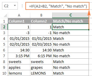
Combining Matches and Differences

You can also combine both matches and differences in a single formula:

=IF(A2=B2,"Match","No match")

Or:

=IF(A2<>B2,"No match","Match")

This provides a clear indication of whether each row contains matching or non-matching values.

2.2. Case-Sensitive Comparisons

The formulas above ignore case when comparing text values. If you need to perform a case-sensitive comparison, use the EXACT function.

Formula for Case-Sensitive Matches

To find case-sensitive matches between two columns, use the following formula:

=IF(EXACT(A2, B2), "Match", "")

This formula compares the values in cells A2 and B2 and returns “Match” only if the values are exactly the same, including case.

Formula for Case-Sensitive Differences

To find case-sensitive differences, use the following formula:

=IF(EXACT(A2, B2), "Match", "Unique")

This formula returns “Match” if the values are exactly the same, and “Unique” if they are different, including case.

3. Comparing Multiple Columns for Matches

When dealing with datasets containing multiple columns, you might need to compare more than two columns at once. Excel provides several ways to achieve this, depending on the specific criteria you want to evaluate.

3.1. Finding Matches in All Cells Within the Same Row

If you want to find rows where all cells have the same values, you can use the AND function in combination with the IF function.

Formula Using AND Function

=IF(AND(A2=B2, A2=C2), "Full match", "")

This formula checks if the values in cells A2, B2, and C2 are all the same. If they are, the formula returns “Full match”; otherwise, it returns an empty string.

Formula Using COUNTIF Function

For tables with many columns, using the COUNTIF function is a more efficient approach:

=IF(COUNTIF($A2:$E2, $A2)=5, "Full match", "")

In this formula, $A2:$E2 is the range of cells you are comparing, and 5 is the number of columns. The formula counts how many cells in the range are equal to the value in the first cell ($A2). If the count equals the number of columns, it means all cells have the same value, and the formula returns “Full match”.

3.2. Finding Matches in Any Two Cells in the Same Row

If you need to identify rows where at least two cells have the same value, you can use the OR function in combination with the IF function.

Formula Using OR Function

=IF(OR(A2=B2, B2=C2, A2=C2), "Match", "")

This formula checks if any two of the cells A2, B2, and C2 have the same value. If at least two cells match, the formula returns “Match”; otherwise, it returns an empty string.

Formula Using COUNTIF Functions

For a larger number of columns, using multiple COUNTIF functions is more manageable:

=IF(COUNTIF(B2:D2,A2)+COUNTIF(C2:D2,B2)+(C2=D2)=0,"Unique","Match")

This formula counts how many columns have the same value as the first column, then counts how many of the remaining columns are equal to the second column, and so on. If the total count is 0, it means no two cells have the same value, and the formula returns “Unique”; otherwise, it returns “Match”.

4. Comparing Two Columns for Matches and Differences Across Entire Lists

Sometimes, you need to compare two columns to find values that exist in one column but not the other. This is useful for identifying unique entries or missing data.

4.1. Using IF and COUNTIF Functions

To find values in column A that do not exist in column B, you can use the COUNTIF function within an IF statement.

=IF(COUNTIF($B:$B, $A2)=0, "No match in B", "")

This formula searches the entire column B for the value in cell A2. If no match is found (i.e., the count is 0), the formula returns “No match in B”; otherwise, it returns an empty string.

4.2. Using IF, ISERROR, and MATCH Functions

Alternatively, you can use the ISERROR and MATCH functions to achieve the same result:

=IF(ISERROR(MATCH($A2,$B$2:$B$10,0)),"No match in B","")

This formula uses the MATCH function to find the position of the value in cell A2 within the range $B$2:$B$10. If the value is not found, MATCH returns an error, which ISERROR detects, causing the formula to return “No match in B”.

4.3. Using Array Formulas

Array formulas offer another way to compare two columns for matches and differences. Note that array formulas need to be entered using Ctrl + Shift + Enter.

=IF(SUM(--($B$2:$B$10=$A2))=0, " No match in B", "")

This formula checks if the sum of all matches in column B for the value in A2 is 0. If it is, the formula returns “No match in B”.

4.4. Identifying Both Matches and Differences

To identify both matches and differences in a single formula, you can modify the IF statement to provide different outputs for each case:

=IF(COUNTIF($B:$B, $A2)=0, "No match in B", "Match in B")

This formula returns “No match in B” if the value in A2 is not found in column B, and “Match in B” if it is found.

5. Pulling Matches from Two Lists

In some scenarios, you may need to not only identify matches between two columns but also retrieve corresponding data from the matching entries. Excel offers several functions to accomplish this, including VLOOKUP, INDEX MATCH, and XLOOKUP.

5.1. Using VLOOKUP Function

The VLOOKUP function is a classic tool for looking up values in a table and returning a corresponding value from another column.

=VLOOKUP(D2, $A$2:$B$6, 2, FALSE)

This formula searches for the value in cell D2 within the range $A$2:$B$6. If a match is found in column A, the formula returns the corresponding value from column B (the second column in the range). The FALSE argument ensures an exact match.

5.2. Using INDEX MATCH Function

The INDEX MATCH combination is a more flexible alternative to VLOOKUP. It allows you to look up values based on both row and column positions.

=INDEX($B$2:$B$6, MATCH($D2, $A$2:$A$6, 0))

This formula first uses the MATCH function to find the row number of the value in cell D2 within the range $A$2:$A$6. Then, it uses the INDEX function to return the value from the range $B$2:$B$6 at the found row number.

5.3. Using XLOOKUP Function

The XLOOKUP function is a more recent addition to Excel, available in Excel 2021 and Excel 365. It combines the capabilities of VLOOKUP and INDEX MATCH with improved flexibility and ease of use.

=XLOOKUP(D2, $A$2:$A$6, $B$2:$B$6)

This formula searches for the value in cell D2 within the range $A$2:$A$6 and returns the corresponding value from the range $B$2:$B$6.

6. Highlighting Matches and Differences Using Conditional Formatting

Conditional formatting is a powerful feature in Excel that allows you to visually highlight cells based on specific criteria. This can be particularly useful when comparing columns of data, as it helps you quickly identify matches and differences.

6.1. Highlighting Matches and Differences in Each Row

To compare two columns and highlight cells in column A that have identical entries in column B in the same row, follow these steps:

Select the cells you want to highlight (e.g., cells in column A).
Go to Conditional Formatting > New Rule… > Use a formula to determine which cells to format.
Enter the following formula:
```
=$B2=$A2
```
This formula compares the value in cell B2 with the value in cell A2. If they are equal, the conditional formatting rule will be applied to cell A2.

To highlight differences between column A and B, create a rule with this formula:

=$B2<>$A2

6.2. Highlighting Unique Entries in Each List

To highlight unique entries in each list, you can use conditional formatting with the COUNTIF function.

Select the cells in List 1 (e.g., $A$2:$A$6).
Go to Conditional Formatting > New Rule… > Use a formula to determine which cells to format.
Enter the following formula:
```
=COUNTIF($C$2:$C$5, $A2)=0
```
This formula checks if the value in cell A2 is not found in the range $C$2:$C$5. If it is not found, the conditional formatting rule will be applied to cell A2.
Repeat the process for List 2 (e.g., $C$2:$C$5) with the following formula:
```
=COUNTIF($A$2:$A$6, $C2)=0
```

6.3. Highlighting Matches (Duplicates) Between Two Columns

To highlight matches between two columns, you can adjust the COUNTIF formulas to find the values that exist in both lists.

Select the cells in List 1 (e.g., $A$2:$A$6).
Go to Conditional Formatting > New Rule… > Use a formula to determine which cells to format.
Enter the following formula:
```
=COUNTIF($C$2:$C$5, $A2)>0
```
This formula checks if the value in cell A2 is found in the range $C$2:$C$5. If it is found, the conditional formatting rule will be applied to cell A2.
Repeat the process for List 2 (e.g., $C$2:$C$5) with the following formula:
```
=COUNTIF($A$2:$A$6, $C2)>0
```

7. Highlighting Row Differences and Matches in Multiple Columns

When working with multiple columns, you might need to highlight entire rows based on whether they contain matching or different values.

7.1. Highlighting Rows with Identical Values in All Columns

To highlight rows that have identical values in all columns, create a conditional formatting rule based on one of the following formulas:

=AND($A2=$B2, $A2=$C2)

Or:

=COUNTIF($A2:$C2, $A2)=3

Where A2, B2, and C2 are the top-most cells, and 3 is the number of columns to compare.

7.2. Highlighting Row Differences

To quickly highlight cells with different values in each individual row, you can use Excel’s Go To Special feature.

Select the range of cells you want to compare.
Go to Home tab, then Editing group, and click Find & Select > Go To Special….
Select Row differences and click the OK button.

The cells whose values are different from the comparison cell in each row will be highlighted. You can then apply a fill color to shade these cells.

8. Comparing Two Individual Cells

Comparing two individual cells is a simplified version of comparing two columns row-by-row. You can use the IF function to check if two cells match or differ.

8.1. Formula for Matches

=IF(A1=C1, "Match", "")

This formula compares the values in cells A1 and C1. If the values are the same, the formula returns “Match”; otherwise, it returns an empty string.

8.2. Formula for Differences

=IF(A1<>C1, "Difference", "")

This formula compares the values in cells A1 and C1. If the values are different, the formula returns “Difference”; otherwise, it returns an empty string.

9. Formula-Free Way to Compare Two Columns/Lists in Excel

For users who prefer a formula-free approach, several third-party add-ins can simplify the process of comparing columns and lists in Excel. These tools often provide a user-friendly interface and additional features such as highlighting matches and differences.

9.1. Using the Compare Two Tables Add-In

One such tool is the Compare Two Tables add-in, which is included in the Ultimate Suite for Excel. This add-in allows you to compare two tables or lists by any number of columns and both identify matches/differences and highlight them.

To compare two lists using this add-in, follow these steps:

Click the Compare Tables button on the Ablebits Data tab.
Select the first column/list and click Next.
Select the second column/list and click Next.
Choose whether to look for duplicate values (matches) or unique values (differences).
Select the columns for comparison.
Choose how to deal with the found items, such as highlighting with color or identifying in a status column.

10. Best Practices for Comparing Values in Excel

To ensure accurate and efficient value comparison in Excel, follow these best practices:

Understand Your Data: Before comparing values, take the time to understand the structure and content of your datasets.
Use Consistent Formatting: Ensure that the data you are comparing is formatted consistently, especially for dates and numbers.
Test Your Formulas: Always test your formulas on a small sample of data to ensure they are working correctly.
Use Absolute and Relative References Appropriately: Understand when to use absolute ($) and relative references in your formulas to avoid errors when copying formulas to other cells.
Handle Errors Gracefully: Use error-handling functions like IFERROR to handle potential errors in your formulas.
Document Your Work: Add comments to your formulas and conditional formatting rules to explain what they do.

11. FAQ: Comparing Values in Excel and Highlighting Differences

Q1: How do I compare two columns in Excel for exact matches?

A1: Use the formula =IF(EXACT(A2, B2), "Match", "") to perform a case-sensitive comparison and identify exact matches.

Q2: Can I compare more than two columns at once?

A2: Yes, you can use formulas like =IF(AND(A2=B2, A2=C2), "Full match", "") or =IF(COUNTIF($A2:$E2, $A2)=5, "Full match", "") to compare multiple columns.

Q3: How can I highlight differences between two columns in Excel?

A3: Use conditional formatting with the formula =$B2<>$A2 to highlight cells in column A that are different from their corresponding cells in column B.

Q4: What is the best way to find unique entries in two lists?

A4: Use conditional formatting with the formula =COUNTIF($C$2:$C$5, $A2)=0 to highlight unique entries in List 1 and =COUNTIF($A$2:$A$6, $C2)=0 for List 2.

Q5: How do I pull matching data from one list to another?

A5: Use the VLOOKUP, INDEX MATCH, or XLOOKUP functions to search for matching values and retrieve corresponding data from another column.

Q6: Is there a formula-free way to compare columns in Excel?

A6: Yes, you can use third-party add-ins like the Compare Two Tables add-in to simplify the comparison process.

Q7: How can I highlight rows with identical values in multiple columns?

A7: Use conditional formatting with formulas like =AND($A2=$B2, $A2=$C2) or =COUNTIF($A2:$C2, $A2)=3.

Q8: Can I use conditional formatting to highlight matches between two columns?

A8: Yes, use conditional formatting with the formula =COUNTIF($C$2:$C$5, $A2)>0 to highlight matches in List 1 and =COUNTIF($A$2:$A$6, $C2)>0 for List 2.

Q9: How do I compare two individual cells in Excel?

A9: Use the formula =IF(A1=C1, "Match", "") to check if two cells match or =IF(A1<>C1, "Difference", "") to check for differences.

Q10: What should I do if my formulas are not working correctly?

A10: Double-check your formulas for errors, ensure that you are using the correct cell references, and test your formulas on a small sample of data.

12. Conclusion

Comparing values in Excel and highlighting differences is a critical skill for data analysis. By mastering the techniques and formulas discussed in this guide, you can efficiently identify matches, differences, and unique entries in your datasets. Whether you prefer using built-in functions, conditional formatting, or third-party add-ins, Excel offers a wide range of tools to streamline your data comparison tasks.

Ready to take your Excel skills to the next level? Visit COMPARE.EDU.VN for more in-depth tutorials, expert tips, and resources to enhance your data analysis capabilities. Make informed decisions and drive success with our comprehensive guides and tools.

For further assistance, contact us at:

Address: 333 Comparison Plaza, Choice City, CA 90210, United States
WhatsApp: +1 (626) 555-9090
Website: compare.edu.vn

Start exploring and comparing data effectively today!