Comparing two columns in Excel is a common task, and compare.edu.vn provides a powerful solution: VLOOKUP. This guide will comprehensively show you how to compare columns, find matches, identify missing data, and return associated values using VLOOKUP and other Excel functions. Discover advanced techniques and alternatives to streamline your data analysis.
1. Understanding the Basics of VLOOKUP for Column Comparison
The VLOOKUP function is a powerful tool in Excel for comparing two columns. VLOOKUP, short for Vertical Lookup, searches for a specific value in the first column of a range and then returns a value from any cell on the same row of that range. It is widely used for various tasks from cross-referencing data to enriching datasets. To effectively use VLOOKUP, understanding its syntax and arguments is crucial.
1.1. Syntax and Arguments of VLOOKUP
The syntax of the VLOOKUP function is as follows:
VLOOKUP(lookup_value, table_array, col_index_num, [range_lookup])
Let’s break down each argument:
- lookup_value: The value you want to search for. This could be a cell reference, a number, text string, or even the result of another formula. In the context of comparing two columns, the lookup_value will typically be a cell from the column you are using as the basis for comparison.
- table_array: The range of cells where you want to search for the lookup_value and from which you want to retrieve a corresponding value. The first column of this range is where VLOOKUP will look for the lookup_value. It’s important to use absolute references (e.g., $A$1:$B$10) for the table_array to prevent it from shifting when you copy the formula to other cells.
- col_index_num: The column number within the table_array from which the matching value will be returned. The first column in the table_array is column 1, the second column is column 2, and so on.
- range_lookup: An optional argument that specifies whether you want an exact match or an approximate match.
- TRUE (or omitted): VLOOKUP will look for an approximate match. The first column in the table_array must be sorted in ascending order. If an exact match is not found, VLOOKUP will return the next largest value that is less than lookup_value.
- FALSE: VLOOKUP will look for an exact match. The first column in the table_array does not need to be sorted. If an exact match is not found, VLOOKUP returns the #N/A error.
In most scenarios involving data comparison, you will want to use FALSE for the range_lookup argument to ensure that you only find exact matches.
1.2. How VLOOKUP Works: A Step-by-Step Explanation
-
Initiation: You enter the VLOOKUP formula in a cell, providing all the necessary arguments: the value to look up, the range in which to look, the column number to return a value from, and whether to look for an exact or approximate match.
-
Lookup Value Search: VLOOKUP starts by searching for the lookup_value in the first column of the table_array. It scans down the column until it finds a value that either matches the lookup_value exactly (if range_lookup is set to FALSE) or is the closest match without exceeding it (if range_lookup is set to TRUE).
-
Match Found:
- Exact Match (range_lookup = FALSE): If VLOOKUP finds an exact match, it notes the row number where the match was found.
- Approximate Match (range_lookup = TRUE): If VLOOKUP finds an approximate match (or the closest value without exceeding), it also notes the row number.
-
Value Retrieval: Once the row number is identified, VLOOKUP moves to the column specified by the col_index_num argument in the same row and retrieves the value from that cell.
-
Result Display: The retrieved value is then displayed in the cell where you entered the VLOOKUP formula.
-
No Match Found: If VLOOKUP does not find a match based on the range_lookup setting:
-
Exact Match (range_lookup = FALSE): VLOOKUP returns the #N/A error, indicating that the lookup_value was not found in the first column of the table_array.
-
Approximate Match (range_lookup = TRUE): VLOOKUP will return the #N/A error if the lookup_value is smaller than the smallest value in the first column of the table_array.
-
1.3. Practical Example of VLOOKUP
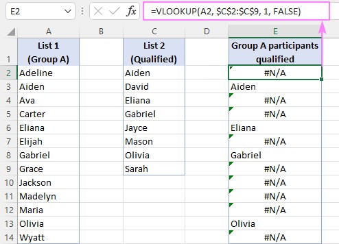
Consider two lists of customer IDs. List 1 is in column A, and List 2 is in column B. You want to determine which customer IDs from List 1 are also present in List 2.
- List 1 (Column A): Contains customer IDs that you want to check against List 2.
- List 2 (Column B): Contains customer IDs that serve as the reference list.
In cell C2, enter the following formula:
=VLOOKUP(A2, $B$2:$B$10, 1, FALSE)
Here’s what each part of the formula does:
- A2: This is the first customer ID in List 1 that you are looking for in List 2.
- $B$2:$B$10: This is the range of cells containing List 2, where VLOOKUP will search for the customer ID. The dollar signs ($) make this an absolute reference, which means it won’t change when you copy the formula to other cells.
- 1: This specifies that if a match is found, VLOOKUP should return the value from the first column of the range $B$2:$B$10, which is the customer ID itself.
- FALSE: This ensures that VLOOKUP only looks for an exact match.
Copy the formula from cell C2 down to the last customer ID in List 1. The results in column C will indicate whether each customer ID from List 1 is present in List 2. If a customer ID is found, the formula will return the customer ID. If a customer ID is not found, the formula will return #N/A.
2. Step-by-Step Guide: Comparing Two Columns Using VLOOKUP
Comparing two columns using VLOOKUP in Excel involves several steps to ensure accuracy and relevance. This section provides a detailed, step-by-step guide to effectively compare two columns and extract meaningful insights.
2.1. Preparing Your Data
Before using VLOOKUP to compare columns, it’s essential to prepare your data correctly. This involves organizing your data in a way that VLOOKUP can efficiently process.
-
Ensure Data Consistency:
-
Data Type: Ensure that the data types in both columns are consistent. For instance, if you’re comparing numbers, both columns should contain numeric data. If comparing text, ensure both are formatted as text. Inconsistent data types can lead to VLOOKUP returning incorrect results or errors.
-
Formatting: Standardize the formatting of data in both columns. Remove any leading or trailing spaces, extra characters, or inconsistencies in capitalization. You can use Excel functions like
TRIM()to remove extra spaces andUPPER()orLOWER()to standardize capitalization.
-
-
Organize Columns:
-
Placement: Place the columns you want to compare side by side, or at least in the same worksheet. This makes it easier to reference them in the VLOOKUP formula.
-
Headers: Add clear and descriptive headers to each column. This not only helps you keep track of the data but also makes it easier for others to understand the spreadsheet.
-
-
Sort Data (If Necessary):
-
Approximate Match: If you plan to use VLOOKUP with an approximate match (i.e., the range_lookup argument is set to TRUE), you must sort the column being searched in ascending order. However, for exact matches, sorting is not required.
-
Sorting: To sort a column, select the data (excluding the header), go to the “Data” tab in Excel, and click on the “Sort” button. Choose the column you want to sort and specify the order (ascending or descending).
-
-
Remove Duplicates (If Necessary):
-
Duplicates: Depending on your analysis goals, you may want to remove duplicate entries from either or both columns. Duplicate entries can skew the results of your comparison.
-
Removing Duplicates: To remove duplicates, select the column, go to the “Data” tab, and click on the “Remove Duplicates” button. Excel will prompt you to select the columns to check for duplicates and then remove any duplicate rows.
-
2.2. Writing the VLOOKUP Formula
After preparing your data, the next step is to write the VLOOKUP formula. This involves understanding the structure of the formula and how to apply it to your specific data set.
-
Identify Lookup Value:
-
Purpose: Determine which column will serve as the basis for the lookup. This is the column from which you will take the values to search for in the other column.
-
Cell Reference: Identify the first cell in the lookup column. This will be the initial lookup_value in your VLOOKUP formula. For example, if your lookup column is column A and you’re starting from the second row, the lookup_value will be A2.
-
-
Define Table Array:
-
Range: Determine the range of cells that contains the column you will be searching for matches in. This range should include the column with the data you want to match against the lookup_value.
-
Absolute References: Use absolute references (e.g., $B$2:$B$10) to define the table_array. This ensures that the range does not change when you copy the formula to other cells. To create an absolute reference, add dollar signs ($) before both the column letter and row number.
-
-
Specify Column Index Number:
-
Column Number: Determine the column number within the table_array from which you want to return a value if a match is found. The first column in the table_array is column 1, the second is column 2, and so on.
-
Purpose: In many cases, when comparing two columns, you might want to return the value from the column where the match is found. If this is the case, and the column you’re searching is the first column in the table_array, the col_index_num will be 1.
-
-
Choose Range Lookup:
-
Exact Match: For most data comparison tasks, you’ll want to use an exact match. This ensures that VLOOKUP only returns a value if it finds an identical match for the lookup_value.
-
Setting to False: Set the range_lookup argument to FALSE. This tells VLOOKUP to look for an exact match.
-
-
Construct the Formula:
- Syntax: Combine all the elements to construct the VLOOKUP formula. The basic syntax is:
=VLOOKUP(lookup_value, table_array, col_index_num, range_lookup)- Example: For instance, if you are looking up values from cell A2 in a table array from $B$2:$B$10 and want to return the value from the first column, the formula would be:
=VLOOKUP(A2, $B$2:$B$10, 1, FALSE)
2.3. Applying the Formula and Interpreting Results
Once you’ve written the VLOOKUP formula, the next step is to apply it to your data and interpret the results. This involves copying the formula down the column and understanding the values and errors that VLOOKUP returns.
-
Enter the Formula:
-
First Cell: Enter the VLOOKUP formula in the first cell where you want the result to appear. This is typically in a column adjacent to your lookup column.
-
Example: If your lookup column is A, you might enter the formula in cell B2.
-
-
Copy the Formula:
-
Drag Down: Copy the formula down to the remaining cells in the column. You can do this by clicking on the bottom-right corner of the cell with the formula (the fill handle) and dragging it down to the last row of your data.
-
Double-Click: Alternatively, you can double-click the fill handle. This will automatically copy the formula down to the last row that contains data in the adjacent column.
-
-
Interpret the Results:
-
Match Found: If VLOOKUP finds a match, it will return the value from the specified column in the table_array. This indicates that the lookup_value exists in the other column.
-
#N/A Error: If VLOOKUP does not find a match, it will return the #N/A error. This means that the lookup_value does not exist in the table_array.
-
-
Handle Errors (Optional):
-
IFERROR Function: To handle the #N/A errors and display a more user-friendly message, you can wrap the VLOOKUP formula inside an
IFERRORfunction. This allows you to specify what value or message should be displayed when VLOOKUP returns an error. -
Syntax: The syntax for the
IFERRORfunction is:
=IFERROR(value, value_if_error)- Example: To display “Not Found” instead of #N/A, use the following formula:
=IFERROR(VLOOKUP(A2, $B$2:$B$10, 1, FALSE), "Not Found")- Blank Cells: To display blank cells instead of #N/A, use an empty string (“”) as the value_if_error:
=IFERROR(VLOOKUP(A2, $B$2:$B$10, 1, FALSE), "") -
-
Filter and Analyze:
-
Filter Results: Use Excel’s filtering capabilities to isolate the matches and non-matches. This allows you to quickly analyze the data and identify any discrepancies.
-
Filtering: To filter the results, select the column with the VLOOKUP formulas, go to the “Data” tab, and click on the “Filter” button. Use the filter dropdown to select the values you want to display (e.g., non-error values or specific error messages).
-
By following these steps, you can effectively compare two columns using VLOOKUP, interpret the results, and handle errors to gain valuable insights from your data.
2.4. Common Issues and Troubleshooting
When comparing two columns using VLOOKUP, you may encounter some common issues. Here are some troubleshooting tips to help you resolve these problems:
-
#N/A Errors:
- Problem: VLOOKUP returns #N/A errors when it cannot find a match for the lookup_value in the table_array.
- Solution:
- Verify Data: Double-check that the lookup_value actually exists in the first column of the table_array.
- Check Spelling: Ensure that there are no spelling errors or typos in either the lookup_value or the values in the table_array.
- Data Types: Make sure that the data types of the lookup_value and the values in the table_array are consistent. For example, if you are comparing numbers, ensure that both are formatted as numbers and not as text.
- Extra Spaces: Remove any leading or trailing spaces from the lookup_value or the values in the table_array. Use the
TRIM()function to remove extra spaces. - Exact Match: Ensure that the range_lookup argument is set to FALSE for an exact match. If it is set to TRUE, VLOOKUP may return an approximate match, which may not be what you want.
-
Incorrect Results:
- Problem: VLOOKUP returns a value, but it is not the correct value.
- Solution:
- Column Index: Verify that the col_index_num argument is correct. It should specify the column number within the table_array from which you want to return a value.
- Table Array: Ensure that the table_array is defined correctly and includes all the necessary columns.
- Absolute References: Use absolute references ($) for the table_array to prevent it from changing when you copy the formula to other cells.
- Data Sorting: If you are using an approximate match (i.e., range_lookup is set to TRUE), make sure that the first column of the table_array is sorted in ascending order.
-
Formula Not Copying Correctly:
- Problem: When you copy the VLOOKUP formula to other cells, the table_array range shifts, causing incorrect results.
- Solution:
- Absolute References: Use absolute references ($) for the table_array to prevent it from changing when you copy the formula. For example, use
$B$2:$B$10instead ofB2:B10.
- Absolute References: Use absolute references ($) for the table_array to prevent it from changing when you copy the formula. For example, use
-
Performance Issues:
- Problem: VLOOKUP is slow when working with large datasets.
- Solution:
- Optimize Data: Remove any unnecessary rows or columns from your dataset.
- Use INDEX and MATCH: Consider using the
INDEXandMATCHfunctions as an alternative to VLOOKUP. TheINDEXandMATCHfunctions can sometimes be faster than VLOOKUP, especially when working with large datasets. - Excel Tables: Convert your data range into an Excel Table (Insert > Table). Tables can improve performance and make your formulas more readable.
3. Advanced VLOOKUP Techniques for Data Comparison
While the basic VLOOKUP function is useful for simple column comparisons, advanced techniques can significantly enhance its capabilities. This section explores several advanced VLOOKUP techniques that can help you tackle more complex data comparison tasks.
3.1. Using VLOOKUP with Multiple Criteria
In some scenarios, you may need to compare columns based on multiple criteria. The VLOOKUP function, by itself, cannot handle multiple criteria directly. However, you can combine VLOOKUP with other Excel functions to achieve this.
-
Concatenate Columns:
-
Combine Criteria: Create a new column in both tables that concatenates the columns containing the criteria you want to match. This creates a unique key that VLOOKUP can use to find matches.
-
Formula: Use the
&operator or theCONCATENATEfunction to combine the columns. For example, if you want to combine columns A and B, the formula would be:
=A2&B2or=CONCATENATE(A2, B2) -
-
Apply VLOOKUP:
-
Lookup Value: Use the concatenated column in the first table as the lookup_value in your VLOOKUP formula.
-
Table Array: Use the concatenated column in the second table as the first column of the table_array.
-
Example: If you have two tables, Table 1 (columns A and B concatenated in column C) and Table 2 (columns D and E concatenated in column F), and you want to find matches from Table 1 in Table 2, the VLOOKUP formula would be:
=VLOOKUP(C2, $F$2:$G$10, 2, FALSE) -
In this example, column G contains additional data from Table 2 that you want to retrieve if a match is found.
3.2. VLOOKUP with Wildcards for Partial Matches
Sometimes, you may need to find partial matches when comparing two columns. VLOOKUP supports the use of wildcards to achieve this.
-
Wildcard Characters:
-
Asterisk (*): Represents any sequence of characters.
-
Question Mark (?): Represents any single character.
-
-
Using Wildcards in VLOOKUP:
-
Lookup Value: Include the wildcard characters in the lookup_value to find partial matches.
-
Example: If you want to find any value in the table_array that starts with “ABC”, the VLOOKUP formula would be:
=VLOOKUP("ABC*", $B$2:$B$10, 1, FALSE)- Partial Match with Question Mark: To find any value that has “ABC” followed by any single character, the formula would be:
=VLOOKUP("ABC?", $B$2:$B$10, 1, FALSE) -
3.3. Returning Multiple Values with VLOOKUP
VLOOKUP is designed to return a single value from a specified column in the table_array. However, you can use multiple VLOOKUP formulas to return multiple values.
-
Multiple VLOOKUPs:
-
Separate Formulas: Use a separate VLOOKUP formula for each column from which you want to return a value.
-
Adjust Column Index: Adjust the col_index_num argument in each VLOOKUP formula to specify the correct column.
-
Example: If you have a table_array in columns B:D and you want to return values from columns C and D, the formulas would be:
=VLOOKUP(A2, $B$2:$D$10, 2, FALSE)(returns value from column C)=VLOOKUP(A2, $B$2:$D$10, 3, FALSE)(returns value from column D) -
3.4. Combining VLOOKUP with INDEX and MATCH
The INDEX and MATCH functions provide a more flexible alternative to VLOOKUP. Combining INDEX and MATCH allows you to perform more complex lookups and overcome some of the limitations of VLOOKUP.
-
MATCH Function:
-
Purpose: The
MATCHfunction finds the position of a lookup_value in a range. -
Syntax:
=MATCH(lookup_value, lookup_array, [match_type]) -
-
INDEX Function:
-
Purpose: The
INDEXfunction returns a value from a specified row and column in a range. -
Syntax:
=INDEX(array, row_num, [column_num]) -
-
Combining INDEX and MATCH:
-
Dynamic Lookup: Use
MATCHto find the row number of the lookup_value and then useINDEXto return a value from that row in the desired column. -
Formula:
=INDEX(return_column, MATCH(lookup_value, lookup_column, 0))- Example: If you want to find the value in column C that corresponds to a lookup_value in column A, the formula would be:
=INDEX($C$2:$C$10, MATCH(A2, $A$2:$A$10, 0)) -
3.5. Comparing Columns with Different Lengths
When comparing columns of different lengths, VLOOKUP can still be used effectively, but you need to ensure that the table_array covers the entire range of the longer column.
-
Dynamic Table Array:
-
Adjust Range: Define the table_array to cover the entire range of the longer column. This ensures that VLOOKUP searches through all possible matches.
-
Example: If column A has 100 rows and column B has 150 rows, the VLOOKUP formula would be:
=VLOOKUP(A2, $B$2:$B$150, 1, FALSE) -
-
Handling Errors:
-
IFERROR Function: Use the
IFERRORfunction to handle any #N/A errors that occur when the lookup_value is not found in the table_array. -
Example:
=IFERROR(VLOOKUP(A2, $B$2:$B$150, 1, FALSE), "Not Found") -
By mastering these advanced VLOOKUP techniques, you can handle a wide range of data comparison tasks with greater flexibility and precision. Whether you need to compare columns based on multiple criteria, find partial matches, return multiple values, or handle columns of different lengths, these techniques will help you unlock the full potential of VLOOKUP.
4. Alternative Methods for Comparing Columns in Excel
While VLOOKUP is a powerful tool for comparing columns in Excel, it’s not the only option. Excel offers several alternative methods that may be more suitable depending on the specific task and dataset. This section explores some of these alternatives, including their strengths and weaknesses, to provide a comprehensive understanding of column comparison techniques in Excel.
4.1. Using the MATCH Function
The MATCH function is a versatile tool for finding the position of a value in a range. Unlike VLOOKUP, which returns a value from a specified column, MATCH returns the relative position of the matched item in the range.
-
Syntax:
=MATCH(lookup_value, lookup_array, [match_type])- lookup_value: The value you want to find.
- lookup_array: The range of cells to search in.
- match_type: Optional. Specifies how Excel matches lookup_value with values in lookup_array. 0 for exact match, 1 for less than, -1 for greater than.
-
Comparing Columns with MATCH:
- Exact Match: To compare two columns and find exact matches, set the match_type argument to 0.
- Formula:
=MATCH(A2, $B$2:$B$10, 0)- Interpretation: If
MATCHfinds a match, it returns the position of the matched value in the lookup_array. If it does not find a match, it returns the #N/A error.
-
Advantages:
- Simplicity:
MATCHis simpler than VLOOKUP and easier to understand. - Flexibility:
MATCHcan be used withINDEXto perform more complex lookups.
- Simplicity:
-
Disadvantages:
- Limited Functionality:
MATCHonly returns the position of the matched value, not the value itself. - Error Handling: Requires additional functions like
IFERRORto handle #N/A errors.
- Limited Functionality:
4.2. Using Conditional Formatting
Conditional formatting allows you to highlight cells based on specific criteria. This can be a useful tool for visually comparing two columns and identifying differences or matches.
-
Highlighting Matches:
- Select Column: Select the first column you want to compare.
- Conditional Formatting: Go to the “Home” tab, click on “Conditional Formatting,” and select “New Rule.”
- Use a Formula: Choose “Use a formula to determine which cells to format.”
- Formula: Enter the following formula:
=COUNTIF($B$2:$B$10, A2)>0- Format: Click on the “Format” button and choose a formatting style (e.g., fill color) to highlight the matches.
- Apply: Click “OK” to apply the conditional formatting rule.
-
Highlighting Differences:
- Select Column: Select the first column you want to compare.
- Conditional Formatting: Go to the “Home” tab, click on “Conditional Formatting,” and select “New Rule.”
- Use a Formula: Choose “Use a formula to determine which cells to format.”
- Formula: Enter the following formula:
=COUNTIF($B$2:$B$10, A2)=0- Format: Click on the “Format” button and choose a formatting style (e.g., fill color) to highlight the differences.
- Apply: Click “OK” to apply the conditional formatting rule.
-
Advantages:
- Visual Comparison: Provides a visual way to compare two columns and identify matches or differences.
- Easy to Use: Conditional formatting is relatively easy to set up and apply.
-
Disadvantages:
- Limited Functionality: Does not provide detailed information about the matches or differences.
- Manual Analysis: Requires manual analysis to interpret the highlighted cells.
4.3. Using the COUNTIF Function
The COUNTIF function counts the number of cells in a range that meet a specified criterion. This can be used to compare two columns and determine how many times a value from one column appears in the other.
-
Syntax:
=COUNTIF(range, criteria)- range: The range of cells you want to count.
- criteria: The criteria that determine which cells to count.
-
Comparing Columns with COUNTIF:
- Count Matches: To count the number of times a value from column A appears in column B, enter the following formula in column C:
=COUNTIF($B$2:$B$10, A2)- Interpretation: The formula returns the number of times the value in cell A2 appears in the range B2:B10.
-
Advantages:
- Simple and Direct:
COUNTIFis simple and direct, making it easy to use. - Numerical Results: Provides numerical results that can be easily analyzed.
- Simple and Direct:
-
Disadvantages:
- Limited Functionality: Only counts the number of matches, does not provide detailed information about the matches.
- Requires Additional Analysis: Requires additional analysis to interpret the results.
4.4. Using the IF Function with ISNUMBER and MATCH
Combining the IF, ISNUMBER, and MATCH functions allows you to compare two columns and return a specified value based on whether a match is found.
-
Formula:
=IF(ISNUMBER(MATCH(A2, $B$2:$B$10, 0)), "Match", "No Match")- MATCH: The
MATCHfunction finds the position of the value in cell A2 in the range B2:B10. - ISNUMBER: The
ISNUMBERfunction checks if the result of theMATCHfunction is a number (i.e., a match was found). - IF: The
IFfunction returns “Match” if a match was found and “No Match” if no match was found.
- MATCH: The
-
Advantages:
- Clear Results: Provides clear “Match” or “No Match” results.
- Easy to Understand: The formula is relatively easy to understand and interpret.
-
Disadvantages:
- Limited Information: Only provides information about whether a match was found, not the value of the match or its position.
- Requires Multiple Functions: Requires combining multiple functions, which can be more complex than using a single function.
4.5. Using Power Query
Power Query is a powerful data transformation and analysis tool in Excel. It can be used to compare two columns and perform a variety of data manipulation tasks.
-
Import Data:
- From Table/Range: Import the two columns into Power Query by selecting the data range and clicking “From Table/Range” in the “Data” tab.
-
Merge Queries:
- Merge: In the Power Query Editor, select one of the queries, go to “Home” > “Merge Queries.”
- Select Columns: Select the columns you want to compare in both queries.
- Join Kind: Choose the appropriate join kind (e.g., “Left Outer” to keep all rows from the first table and matching rows from the second table).
-
Expand Columns:
- Expand: Expand the columns from the second table to see the matching values.
-
Advantages:
- Powerful Data Transformation: Power Query offers powerful data transformation capabilities.
- Flexible Joins: Supports various join types to handle different comparison scenarios.
- Automation: Allows you to automate the data comparison process.
-
Disadvantages:
- Complexity: Power Query can be more complex to use than other methods.
- Learning Curve: Requires a learning curve to master Power Query.
Each of these alternative methods offers unique advantages and disadvantages for comparing columns in Excel. The best method to use depends on the specific task, the size of the dataset, and the level of detail required. By understanding these alternatives, you can choose the most efficient and effective method for your data comparison needs.
5. Real-World Applications of Comparing Columns Using VLOOKUP
Comparing columns using VLOOKUP and other Excel techniques has numerous real-world applications across various industries and business functions. This section explores several practical examples of how these techniques can be used to solve common problems and improve decision-making.
5.1. Data Validation and Cleansing
Data validation and cleansing are critical processes for ensuring the accuracy and reliability of data. Comparing columns can be a valuable tool for identifying and correcting errors in datasets.
-
Identifying Invalid Data:
- Scenario: A company maintains a list of customer IDs in one system and a list of valid product codes in another. They need to ensure that all customer records are associated with valid product codes.
- Solution:
- VLOOKUP: Use VLOOKUP to compare the product codes in the customer records against the list of valid product codes.
- Error Handling: Use IFERROR to identify any invalid product codes.
- Correction: Correct or remove the invalid product codes to ensure data integrity.
-
Checking Data Consistency:
- Scenario: A marketing team needs to ensure that customer email addresses are consistent across multiple databases.
- Solution:
- VLOOKUP: Use VLOOKUP to compare email addresses from different databases.
- Highlight Differences: Use conditional formatting to highlight any inconsistencies.
- Update Records: Update the inconsistent email addresses to ensure data consistency.
5.2. Inventory Management
Effective inventory management is essential for businesses to optimize stock levels, reduce costs, and meet customer demand. Comparing columns can help streamline inventory processes.
-
Reconciling Inventory Records:
- Scenario: A retail company needs to reconcile inventory records between their warehouse management system (WMS) and their accounting system.
- Solution:
- VLOOKUP: Use VLOOKUP to compare the list of items in the WMS against the list in the accounting system.
- Identify Discrepancies: Identify any discrepancies in item quantities or descriptions.
- Investigate and Correct: Investigate and correct the discrepancies to ensure accurate inventory records.
-
Identifying Obsolete Inventory:
- Scenario: A manufacturing company needs to identify obsolete inventory items that are no longer in production.
- Solution:
- VLOOKUP: Use VLOOKUP to compare the list of inventory items against the list of active product codes.
- Flag Obsolete Items: Flag any inventory items that are not