Comparing Excel columns for differences is a common task in data analysis. At COMPARE.EDU.VN, we provide comprehensive guides and tools to help you efficiently identify discrepancies between columns. Discover simple yet powerful methods to highlight differences and ensure data integrity.
Are you struggling to identify differences between columns in Excel? COMPARE.EDU.VN offers a comprehensive guide to help you quickly and accurately compare data, find unmatched entries, and improve your spreadsheet analysis. Learn effective techniques using formulas and conditional formatting to streamline your workflow and ensure data accuracy. Explore advanced methods for complex comparisons and discover tips for efficient data management, including tools for data validation, auditing, and cleaning that can greatly enhance your data handling capabilities.
1. Understanding the Need to Compare Columns in Excel
Comparing columns in Excel is essential for data validation, ensuring accuracy, and identifying inconsistencies across datasets. Businesses and individuals alike rely on Excel for organizing and analyzing information, making the ability to compare columns a crucial skill. According to a study by the University of California, Berkeley, errors in spreadsheets affect approximately 25% of all companies, leading to significant financial losses. This highlights the importance of accurate data comparison techniques.
- Data Validation: Verify data accuracy by comparing against a known standard.
- Error Detection: Identify errors and inconsistencies in datasets.
- Change Tracking: Monitor changes and updates over time.
- Duplicate Identification: Find and remove duplicate entries.
- Data Cleansing: Ensure data integrity for reliable analysis.
2. Key Search Intents for Comparing Excel Columns
Understanding user intent is crucial for providing relevant and helpful content. Here are five key search intents related to comparing Excel columns:
- Find Differences: Users want to identify unique entries in two columns.
- Find Matches: Users want to find common entries in two columns.
- Row-by-Row Comparison: Users need to compare data in corresponding rows.
- Highlight Differences: Users want to visually identify discrepancies.
- Formula-Free Methods: Users seek easier, non-formula based solutions.
3. Essential Excel Functions for Column Comparison
Excel provides several functions that are instrumental in comparing columns effectively. These include IF, COUNTIF, MATCH, and ISERROR.
-
IF Function: Performs logical tests and returns different values based on whether the test is true or false.
=IF(A1=B1, "Match", "No Match") -
COUNTIF Function: Counts the number of cells within a range that meet a given criteria.
=COUNTIF(B:B, A1) -
MATCH Function: Searches for a specified item in a range of cells, and then returns the relative position of that item in the range.
=MATCH(A1, B:B, 0) -
ISERROR Function: Checks whether a value is an error, and returns TRUE or FALSE.
=ISERROR(MATCH(A1, B:B, 0))
Using these functions, you can perform various types of comparisons, from simple matching to complex conditional analyses.
4. Step-by-Step Guide: How to Compare Two Columns Row-by-Row
Comparing two columns row-by-row is a common task in Excel. The IF function is your best friend here.
4.1. Using the IF Function for Direct Comparison
The IF function allows you to compare corresponding cells in two columns and return a specified value if the condition is met (or not met).
-
Open your Excel sheet: Ensure you have your data ready in two columns.
-
Select a cell: Choose an empty column where you want the results to appear.
-
Enter the formula: In the first cell of the results column (e.g., C2), enter the following formula:
=IF(A2=B2, "Match", "No Match")Here, A2 and B2 are the first cells in the two columns you want to compare.
-
Drag the fill handle: Click and drag the small square at the bottom-right of the cell down to apply the formula to the rest of the rows.
4.2. Handling Case Sensitivity
By default, Excel is not case-sensitive. If you need to perform a case-sensitive comparison, use the EXACT function within the IF function:
=IF(EXACT(A2, B2), "Match", "No Match")
The EXACT function checks if two text strings are identical, including case.
4.3. Example Scenario
Imagine you have two columns, A and B, containing customer names. You want to check if the names are identical in both columns:
| Column A | Column B | Column C (Result) | |
|---|---|---|---|
| Row 1 | Name | Name | Status |
| Row 2 | John Doe | John Doe | Match |
| Row 3 | Jane Smith | Jane Smith | Match |
| Row 4 | Peter Jones | Peter Joness | No Match |
Using the formula =IF(A2=B2, "Match", "No Match") in column C, you can quickly identify matches and discrepancies.
5. Comparing Multiple Columns for Matches
When you need to compare more than two columns, you can use a combination of IF and AND functions or the COUNTIF function.
5.1. Using IF and AND for Multiple Comparisons
If you have three columns (A, B, and C) and want to ensure all values are identical in each row, use the following formula:
=IF(AND(A2=B2, B2=C2), "Match", "No Match")
This formula returns “Match” only if A2 equals B2, and B2 equals C2.
5.2. Using COUNTIF for Efficient Comparison
For comparing many columns, the COUNTIF function is more efficient. For example, to compare five columns (A through E):
=IF(COUNTIF(A2:E2, A2)=5, "Match", "No Match")
This formula checks if the value in A2 appears five times in the range A2:E2, indicating that all columns match.
5.3. Example Scenario
Suppose you have columns A, B, C, and D containing product codes. You want to ensure each code is consistent across all columns:
| Column A | Column B | Column C | Column D | Column E (Result) | |
|---|---|---|---|---|---|
| Row 1 | Code | Code | Code | Code | Status |
| Row 2 | 1234 | 1234 | 1234 | 1234 | Match |
| Row 3 | 5678 | 5678 | 5678 | 5678 | Match |
| Row 4 | 9012 | 9012 | 9012 | 9013 | No Match |
Using the formula =IF(COUNTIF(A2:D2, A2)=4, "Match", "No Match"), you can verify the consistency of the product codes.
6. Comparing Two Columns for Matches and Differences
To identify entries that exist in one column but not the other, you can use the COUNTIF function in combination with the IF function.
6.1. Finding Unique Entries in Column A
To find values in column A that do not exist in column B, use the following formula:
=IF(COUNTIF(B:B, A2)=0, "Unique in A", "")
This formula searches column B for the value in A2. If COUNTIF returns 0 (meaning the value is not found), the formula returns “Unique in A”.
6.2. Finding Unique Entries in Column B
Similarly, to find values in column B that do not exist in column A:
=IF(COUNTIF(A:A, B2)=0, "Unique in B", "")
6.3. Example Scenario
Consider two columns, A and B, listing email addresses of subscribers. You want to find subscribers who are only in one list:
| Column A | Column B | Column C (Result A) | Column D (Result B) | |
|---|---|---|---|---|
| Row 1 | Status A | Status B | ||
| Row 2 | [email protected] | [email protected] | Unique in B | |
| Row 3 | [email protected] | [email protected] | Unique in B | |
| Row 4 | [email protected] | [email protected] | Unique in A |
Using the formulas =IF(COUNTIF(B:B, A2)=0, "Unique in A", "") and =IF(COUNTIF(A:A, B2)=0, "Unique in B", ""), you can identify unique subscribers in each list.
7. How to Compare Two Lists and Pull Matches
Sometimes, you need to not only identify matches but also retrieve corresponding data from the matching entries. The VLOOKUP, INDEX MATCH, and XLOOKUP functions are invaluable for this purpose.
7.1. Using VLOOKUP
VLOOKUP searches for a value in the first column of a range and returns a value in the same row from a column you specify.
=VLOOKUP(D2, $A$2:$B$6, 2, FALSE)
- D2: The value to look up.
- $A$2:$B$6: The range to search in (column A is the lookup column).
- 2: The column number in the range from which to return a value.
- FALSE: Exact match.
7.2. Using INDEX MATCH
INDEX MATCH is a more flexible alternative to VLOOKUP.
=INDEX($B$2:$B$6, MATCH($D2, $A$2:$A$6, 0))
- $B$2:$B$6: The range containing the value to return.
- MATCH($D2, $A$2:$A$6, 0): Finds the position of the lookup value in column A.
7.3. Using XLOOKUP (Excel 365 and Later)
XLOOKUP is the modern successor to VLOOKUP and INDEX MATCH, offering improved functionality and ease of use.
=XLOOKUP(D2, $A$2:$A$6, $B$2:$B$6)
- D2: The lookup value.
- $A$2:$A$6: The lookup range.
- $B$2:$B$6: The return range.
7.4. Example Scenario
Suppose you have a list of product IDs and their corresponding prices in columns A and B. You want to retrieve the price for a specific product ID from column D:
| Column A | Column B | Column D | Column E (Result) | ||
|---|---|---|---|---|---|
| Row 1 | Product ID | Price | Product ID | Price | |
| Row 2 | 1001 | $20 | 1003 | $25 | |
| Row 3 | 1002 | $22 | 1001 | $20 | |
| Row 4 | 1003 | $25 |
Using the formula =XLOOKUP(D2, $A$2:$A$4, $B$2:$B$4), you can retrieve the price for the specified product IDs.
8. Conditional Formatting: Highlight Matches and Differences
Conditional formatting allows you to visually highlight matches and differences between columns, making it easier to spot discrepancies.
8.1. Highlighting Matches
- Select the range: Select the columns you want to compare (e.g., A2:B10).
- Go to Conditional Formatting: Click Home > Conditional Formatting > New Rule.
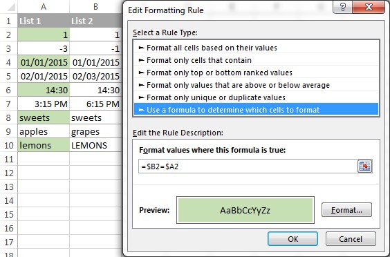
- Use a formula: Select “Use a formula to determine which cells to format.”
- Enter the formula:
- To highlight matches in each row:
=$A2=$B2
- To highlight matches in each row:
- Choose a format: Click Format and select a fill color to highlight matches.
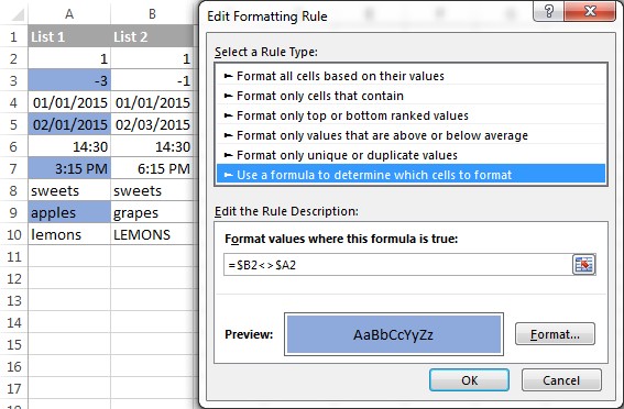
8.2. Highlighting Differences
Follow the same steps as above, but use the following formula to highlight differences:
=$A2<>$B2
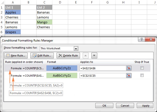
8.3. Highlighting Unique Entries in Each List
- Select List 1 (Column A): Home > Conditional Formatting > New Rule > Use a formula.
- Enter the formula:
=COUNTIF($C$2:$C$5, $A2)=0(assuming List 2 is in C2:C5). - Format: Choose a fill color.
Repeat for List 2 (Column C), using the formula: =COUNTIF($A$2:$A$6, $C2)=0 (assuming List 1 is in A2:A6).
8.4. Example Scenario
Imagine you are comparing two lists of inventory items and want to highlight matches and differences:
| Column A (List 1) | Column B (List 2) | |
|---|---|---|
| Row 1 | Item A | Item A |
| Row 2 | Item B | Item C |
| Row 3 | Item C | Item D |
| Row 4 | Item E | Item F |
Using conditional formatting, you can highlight the matching items (Item A) and the unique items in each list.
9. Highlight Row Differences and Matches in Multiple Columns
For more complex comparisons involving multiple columns, you can use conditional formatting combined with Excel’s “Go To Special” feature.
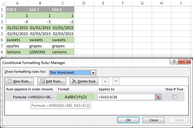
9.1. Highlighting Rows with Identical Values
To highlight rows where all columns have identical values:
- Select the range: Select the data range (e.g., A2:C8).
- Go to Conditional Formatting: Home > Conditional Formatting > New Rule > Use a formula.
- Enter the formula:
AND($A2=$B2, $A2=$C2)orCOUNTIF($A2:$C2, $A2)=3 - Format: Choose a fill color.
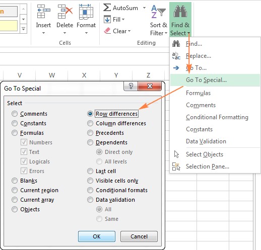
9.2. Highlighting Row Differences Using “Go To Special”
- Select the range: Select the data range (e.g., A2:C8).
- Go to Special: Home > Find & Select > Go To Special.
- Select Row Differences: Choose “Row differences” and click OK.
- Format: The cells with different values will be selected. Click the Fill Color icon to highlight them.
9.3. Example Scenario
Consider a table with product details across multiple columns, such as name, price, and availability. You want to quickly highlight rows with inconsistent information:
| Column A (Name) | Column B (Price) | Column C (Availability) | |
|---|---|---|---|
| Row 1 | Product X | $20 | Available |
| Row 2 | Product Y | $25 | Available |
| Row 3 | Product Z | $30 | Out of Stock |
| Row 4 | Product X | $20 | Out of Stock |
Using the “Go To Special” feature, you can highlight rows where the product name doesn’t match the corresponding price or availability.
10. Comparing Two Cells: A Simplified Approach
Comparing two individual cells is a straightforward process using the IF function.
10.1. Simple Comparison
To compare cells A1 and C1, use the following formulas:
- For Matches:
=IF(A1=C1, "Match", "") - For Differences:
=IF(A1<>C1, "Difference", "")
10.2. Example Scenario
Suppose you have two cells with order numbers and want to quickly verify if they are the same:
| Column A | Column B | Column C (Result) | |
|---|---|---|---|
| Row 1 | Order # | Order # | Status |
| Row 2 | 12345 | 12345 | Match |
| Row 3 | 67890 | 67891 | Difference |
Using the formula =IF(A2=B2, "Match", "Difference"), you can easily check if the order numbers match.
11. Formula-Free Methods: Comparing Columns with Built-in Tools
While formulas provide great flexibility, Excel also offers formula-free methods for comparing columns, particularly through the “Remove Duplicates” feature and the Kutools add-in.
11.1. Using the “Remove Duplicates” Feature
The “Remove Duplicates” feature can help identify common entries between two columns.
- Copy the columns: Copy the two columns into a single column.
- Select the column: Select the entire column with the combined data.
- Remove Duplicates: Go to Data > Remove Duplicates.
- Identify unique entries: The remaining entries are unique to each original column.
11.2. Using Kutools for Excel
Kutools is a third-party add-in that provides additional tools for comparing data in Excel. It offers a user-friendly interface and simplifies complex comparison tasks.
- Install Kutools: Download and install the Kutools add-in.
- Compare Columns: Use the “Compare Columns” feature to quickly identify matches and differences without writing formulas.
11.3. Example Scenario
You have two lists of customer IDs and want to find common IDs without using formulas:
- Copy both lists into one column.
- Use “Remove Duplicates” to eliminate duplicate IDs.
- The remaining IDs are unique to each original list.
12. Leveraging Advanced Features: Power Query for Complex Comparisons
For advanced users dealing with large datasets, Power Query offers robust capabilities for comparing columns.
12.1. Importing Data into Power Query
- Select Data: Select the data range in Excel.
- Go to Data Tab: Click Data > From Table/Range.
- Power Query Editor: The data will open in the Power Query Editor.
12.2. Merging Queries for Comparison
- Home Tab: In the Power Query Editor, click Home > Merge Queries.
- Select Tables: Choose the two tables you want to compare.
- Select Columns: Select the columns to match on.
- Join Kind: Choose the appropriate join kind (e.g., Left Anti to find unique entries in the first table).
- Expand: Expand the merged column to view the results.
12.3. Example Scenario
You have two Excel tables with customer information and want to find customers present in one table but not the other:
- Import both tables into Power Query.
- Merge the queries using a Left Anti join to find unique customers in the first table.
- Load the results back into Excel.
13. Optimizing Performance: Best Practices for Large Datasets
Comparing columns in large datasets can be resource-intensive. Follow these best practices to optimize performance:
- Use Efficient Formulas: Use COUNTIF and MATCH functions judiciously, and consider using INDEX MATCH instead of VLOOKUP for large datasets.
- Avoid Volatile Functions: Minimize the use of volatile functions like NOW() and RAND() as they recalculate with every change, slowing down performance.
- Use Helper Columns: Create helper columns to perform intermediate calculations, which can simplify complex formulas and improve performance.
- Disable Automatic Calculation: Temporarily disable automatic calculation (Formulas > Calculation Options > Manual) when making changes to large datasets, and then manually calculate when needed.
- Use Excel Tables: Convert your data ranges into Excel tables (Insert > Table) to improve performance and manageability.
14. Real-World Examples: Practical Applications of Column Comparison
Column comparison techniques are valuable in various industries and scenarios.
14.1. Financial Analysis
In finance, comparing columns can help reconcile bank statements with internal records, identify discrepancies in transactions, and ensure compliance with regulations.
- Reconciling Bank Statements: Compare transactions listed in bank statements with internal records to identify missing or incorrect entries.
- Auditing Financial Data: Verify the accuracy of financial data by comparing against established standards.
- Detecting Fraudulent Activities: Identify unusual patterns or discrepancies in financial transactions that may indicate fraudulent activity.
14.2. Inventory Management
In inventory management, comparing columns can help track stock levels, identify discrepancies between physical inventory and recorded data, and optimize stock management.
- Tracking Stock Levels: Compare recorded stock levels with physical counts to identify discrepancies.
- Optimizing Stock Management: Identify slow-moving or obsolete items by comparing sales data with inventory levels.
- Ensuring Data Accuracy: Verify the accuracy of inventory data by comparing against established standards.
14.3. Sales and Marketing
In sales and marketing, comparing columns can help analyze customer data, identify trends, and optimize marketing campaigns.
- Analyzing Customer Data: Compare customer data from different sources to create a comprehensive customer profile.
- Identifying Trends: Analyze sales data to identify trends and patterns in customer behavior.
- Optimizing Marketing Campaigns: Compare the results of different marketing campaigns to optimize effectiveness.
15. Common Mistakes to Avoid When Comparing Columns
Avoid these common mistakes to ensure accurate and efficient column comparison:
- Ignoring Case Sensitivity: Remember to use the EXACT function when case sensitivity is important.
- Using Inefficient Formulas: Choose the most efficient formulas for your specific comparison task.
- Not Using Absolute References: Use absolute references ($) to prevent formulas from changing when copied to other cells.
- Not Validating Results: Always validate your results to ensure accuracy.
- Not Handling Errors: Use the IFERROR function to handle errors gracefully.
16. Frequently Asked Questions (FAQ)
1. How can I compare two columns in Excel for partial matches?
Use the SEARCH function within an IF function to find partial matches. For example: =IF(ISNUMBER(SEARCH(A1, B1)), "Partial Match", "No Match")
2. Can I compare two columns in different Excel sheets?
Yes, you can reference cells in different sheets by including the sheet name in the formula. For example: =IF(Sheet1!A1=Sheet2!A1, "Match", "No Match")
3. How do I compare two columns and return a value from a third column if there is a match?
Use the VLOOKUP or INDEX MATCH functions. For example: =VLOOKUP(A1, Sheet2!A:C, 3, FALSE)
4. How can I ignore blank cells when comparing columns?
Use an IF function to check if the cells are blank before comparing. For example: =IF(OR(ISBLANK(A1), ISBLANK(B1)), "", IF(A1=B1, "Match", "No Match"))
5. How can I compare two columns and highlight the entire row if there is a difference?
Use conditional formatting with a formula that references the first cell in the row. For example: =$A1<>$B1
6. What is the best way to compare two large columns in Excel?
Use efficient formulas like COUNTIF or INDEX MATCH, disable automatic calculation, and consider using Power Query for complex comparisons.
7. How do I compare two columns for duplicate values within the same column?
Use the COUNTIF function. For example, to highlight duplicates in column A: =COUNTIF($A:$A, A1)>1
8. Can I compare columns with mixed data types (e.g., text and numbers)?
Excel may treat numbers formatted as text differently. Ensure data types are consistent before comparing.
9. How do I compare two columns and return the differences?
You can use the FILTER function (Excel 365 and later) to return the unique entries.
10. What is the difference between VLOOKUP and INDEX MATCH for comparing columns?
VLOOKUP requires the lookup value to be in the first column of the range, while INDEX MATCH is more flexible and can look up values in any column.
17. Conclusion: Mastering Column Comparison in Excel
Comparing columns in Excel is a critical skill for data analysis and management. Whether you’re using simple formulas like IF and COUNTIF or leveraging advanced features like Power Query, understanding these techniques can significantly improve your efficiency and accuracy. Remember to optimize your approach for large datasets and avoid common mistakes to ensure reliable results. For more detailed comparisons and to make informed decisions, visit COMPARE.EDU.VN, where you’ll find comprehensive comparisons and expert advice.
Ready to streamline your data analysis and make informed decisions? Visit COMPARE.EDU.VN today to explore more comprehensive guides and expert comparisons. Let us help you master Excel and turn your data into actionable insights.
Contact Us:
- Address: 333 Comparison Plaza, Choice City, CA 90210, United States
- WhatsApp: +1 (626) 555-9090
- Website: compare.edu.vn