**How Can You Compare a Participant’s Score to the Mean?**

Comparing a participant’s score to the mean is a fundamental statistical technique used across various fields. COMPARE.EDU.VN provides comprehensive comparisons and analysis to help you understand and interpret these scores effectively, ensuring informed decision-making. By understanding how individual data points deviate from the average, you gain valuable insights into performance, trends, and potential areas for improvement.

1. What Does It Mean to Compare a Participant’s Score to the Mean?

Comparing a participant’s score to the mean involves assessing how much an individual data point deviates from the average or central tendency of a dataset. This comparison is crucial in various fields, including education, healthcare, and business, as it provides insights into individual performance relative to the group. By understanding this deviation, we can identify outliers, evaluate effectiveness, and tailor interventions or strategies more effectively.

1.1. Understanding the Mean

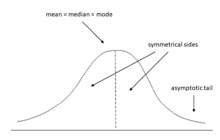
The mean, often referred to as the average, is calculated by summing all the values in a dataset and dividing by the number of values. It represents the central tendency of the data, providing a single value that summarizes the overall distribution.

Formula for the Mean:
[
text{Mean} = frac{sum_{i=1}^{n} x_i}{n}
]
Where:

• ( x_i ) represents each individual value in the dataset.
• ( n ) is the number of values in the dataset.

Example:
Consider the following set of scores: 60, 70, 80, 90, 100.
[
text{Mean} = frac{60 + 70 + 80 + 90 + 100}{5} = frac{400}{5} = 80
]
In this case, the mean score is 80.

1.2. Calculating the Deviation

The deviation is the difference between an individual score and the mean. It indicates how far away a particular data point is from the average.

Formula for Deviation:
[
text{Deviation} = x_i – text{Mean}
]
Where:

• ( x_i ) is the individual score.
• ( text{Mean} ) is the average of the dataset.

Example:
Using the same set of scores (60, 70, 80, 90, 100) with a mean of 80:

• Deviation for 60: ( 60 – 80 = -20 )
• Deviation for 70: ( 70 – 80 = -10 )
• Deviation for 80: ( 80 – 80 = 0 )
• Deviation for 90: ( 90 – 80 = 10 )
• Deviation for 100: ( 100 – 80 = 20 )

These deviations show how each score varies from the mean. Negative values indicate scores below the average, while positive values indicate scores above the average.

1.3. Interpreting the Deviation

The interpretation of the deviation is crucial for understanding the significance of the score relative to the group.

• Positive Deviation: A positive deviation indicates that the participant’s score is above the average. For example, a deviation of 20 means the score is 20 units higher than the mean.
• Negative Deviation: A negative deviation indicates that the participant’s score is below the average. For example, a deviation of -10 means the score is 10 units lower than the mean.
• Zero Deviation: A zero deviation indicates that the participant’s score is exactly at the average.

Example:
In the example above:

• A score of 100 (deviation of 20) is significantly above average.
• A score of 60 (deviation of -20) is significantly below average.
• A score of 80 (deviation of 0) is exactly at the average.

**1.4. The Importance of Context

The interpretation of a score’s deviation from the mean is heavily dependent on context. The same deviation can have different implications depending on the situation.

Example:

• Education: In a classroom setting, a positive deviation might indicate strong performance, while a negative deviation may signal the need for additional support.
• Healthcare: In medical tests, a significant deviation from the mean (either positive or negative) might indicate a health issue requiring further investigation.
• Business: In sales performance, a positive deviation suggests high achievement, whereas a negative deviation may prompt a review of strategies.

Understanding the context ensures that the deviation is interpreted accurately and leads to appropriate actions.

1.5. Limitations of Using the Mean Alone

While the mean provides a valuable measure of central tendency, it has limitations when used in isolation.

• Sensitivity to Outliers: The mean can be heavily influenced by extreme values (outliers), which can distort the representation of the typical score.
• Lack of Information on Variability: The mean does not provide information about the spread or distribution of the scores. Datasets with the same mean can have very different levels of variability.
• Misleading Interpretation: In skewed distributions, the mean may not accurately represent the typical value.

To overcome these limitations, it is essential to use additional statistical measures such as standard deviation, median, and range to gain a more comprehensive understanding of the data. compare.edu.vn can assist in providing these additional measures and interpretations.

2. Why Is Comparing a Score to the Mean Important?

Comparing a score to the mean is important because it provides a standardized way to understand individual performance relative to a larger group, identify outliers, and evaluate the effectiveness of interventions. This comparison is crucial across various fields for making informed decisions and driving improvements.

2.1. Provides a Frame of Reference

Comparing a score to the mean offers a crucial frame of reference, enabling a standardized understanding of individual performance within a group. The mean serves as a benchmark, allowing us to assess whether a score is above, below, or at the average.

Example:
In a company, knowing that a salesperson’s performance is 1.5 standard deviations above the mean provides a clear indication of their exceptional performance compared to their peers.

2.2. Helps Identify Outliers

Identifying outliers is one of the primary reasons for comparing scores to the mean. Outliers are data points that significantly deviate from the average and can indicate unusual events, errors in data collection, or exceptional performance.

Example:
In a manufacturing process, if the average weight of a product is 500 grams, and one item weighs 700 grams, this outlier can signal a malfunction in the machinery or an error in the process.

2.3. Facilitates Performance Evaluation

Comparing scores to the mean is fundamental in performance evaluation across various domains. It helps in assessing individual or group achievements against a standard benchmark.

Example:
In education, comparing a student’s test score to the class average helps evaluate their understanding of the material and identify areas where they may need additional support.

2.4. Enables Data Standardization

Data standardization is essential for comparing scores from different datasets or scales. Transforming scores into z-scores (which measure the number of standard deviations from the mean) allows for meaningful comparisons, regardless of the original scale.

Example:
Comparing scores from two different tests with different scales becomes possible by converting them to z-scores. A student who scores 2 standard deviations above the mean in both tests has performed equally well, despite the tests having different scoring systems.

2.5. Informs Decision-Making

The insights gained from comparing scores to the mean are invaluable in informing decision-making processes across various fields.

Example:
In healthcare, if a patient’s blood pressure reading is significantly above the mean, a doctor can make informed decisions about treatment plans, lifestyle changes, or further diagnostic tests.

2.6. Supports Targeted Interventions

Identifying deviations from the mean allows for targeted interventions, ensuring that resources are allocated effectively to those who need them most.

Example:
In a workplace, if an employee’s performance is significantly below the mean, the manager can provide targeted training, mentorship, or additional resources to help them improve.

2.7. Enhances Predictive Modeling

Comparing scores to the mean can enhance predictive modeling by identifying variables that significantly impact outcomes.

Example:
In marketing, analyzing how customer spending deviates from the mean can help predict future purchasing behavior and tailor marketing campaigns to specific customer segments.

3. How Do You Calculate the Deviation from the Mean?

Calculating the deviation from the mean involves a few straightforward steps. First, you need to determine the mean (average) of your dataset. Then, for each individual data point, subtract the mean from that value. This difference is the deviation. The formula is: Deviation = Individual Value – Mean.

3.1. Step-by-Step Guide to Calculating Deviation from the Mean

To accurately calculate the deviation from the mean, follow these steps:

1. Collect the Data:

   • Gather all the data points in your dataset. Ensure that the data is relevant to the analysis you intend to perform.

   Example:
   Consider a dataset of test scores: 75, 82, 90, 68, 85.

2. Calculate the Mean:

   • Sum all the data points and divide by the number of data points.
     [
     text{Mean} = frac{sum_{i=1}^{n} x_i}{n}
     ]
     Where:
     • ( x_i ) represents each individual value in the dataset.
     • ( n ) is the number of values in the dataset.

   Example:
   [
   text{Mean} = frac{75 + 82 + 90 + 68 + 85}{5} = frac{400}{5} = 80
   ]

3. Calculate the Deviation for Each Data Point:

   • For each data point, subtract the mean from the data point.
     [
     text{Deviation} = x_i – text{Mean}
     ]
     Where:
     • ( x_i ) is the individual data point.
     • ( text{Mean} ) is the average of the dataset.

   Example:

   • Deviation for 75: ( 75 – 80 = -5 )
   • Deviation for 82: ( 82 – 80 = 2 )
   • Deviation for 90: ( 90 – 80 = 10 )
   • Deviation for 68: ( 68 – 80 = -12 )
   • Deviation for 85: ( 85 – 80 = 5 )

4. Interpret the Deviations:

   • Analyze the deviations to understand how each data point varies from the mean.
     • Positive deviations indicate that the data point is above the mean.
     • Negative deviations indicate that the data point is below the mean.
     • A deviation of zero indicates that the data point is equal to the mean.

   Example:

   • A score of 90 has a deviation of 10, indicating it is 10 points above the average.
   • A score of 68 has a deviation of -12, indicating it is 12 points below the average.

3.2. Practical Examples

Let’s apply the calculation of deviation from the mean to different scenarios:

1. Sales Performance:

   • A company wants to analyze the sales performance of its employees. The monthly sales figures (in thousands of dollars) for five employees are: 45, 55, 60, 50, 70.

   • Calculate the Mean:
     [
     text{Mean} = frac{45 + 55 + 60 + 50 + 70}{5} = frac{280}{5} = 56
     ]

   • Calculate the Deviations:

     • Deviation for 45: ( 45 – 56 = -11 )
     • Deviation for 55: ( 55 – 56 = -1 )
     • Deviation for 60: ( 60 – 56 = 4 )
     • Deviation for 50: ( 50 – 56 = -6 )
     • Deviation for 70: ( 70 – 56 = 14 )

   • Interpretation:

     • The employee with sales of $70,000 is performing significantly above average (deviation of 14).
     • The employee with sales of $45,000 is performing significantly below average (deviation of -11).

2. Healthcare Data:

   • A clinic records the waiting times (in minutes) for patients: 20, 25, 30, 15, 40.

   • Calculate the Mean:
     [
     text{Mean} = frac{20 + 25 + 30 + 15 + 40}{5} = frac{130}{5} = 26
     ]

   • Calculate the Deviations:

     • Deviation for 20: ( 20 – 26 = -6 )
     • Deviation for 25: ( 25 – 26 = -1 )
     • Deviation for 30: ( 30 – 26 = 4 )
     • Deviation for 15: ( 15 – 26 = -11 )
     • Deviation for 40: ( 40 – 26 = 14 )

   • Interpretation:

     • A patient who waited 40 minutes experienced a significantly longer wait time compared to the average (deviation of 14).
     • A patient who waited 15 minutes experienced a significantly shorter wait time compared to the average (deviation of -11).

3. Manufacturing Quality Control:

   • A factory measures the weight (in grams) of products: 150, 155, 160, 145, 170.

   • Calculate the Mean:
     [
     text{Mean} = frac{150 + 155 + 160 + 145 + 170}{5} = frac{780}{5} = 156
     ]

   • Calculate the Deviations:

     • Deviation for 150: ( 150 – 156 = -6 )
     • Deviation for 155: ( 155 – 156 = -1 )
     • Deviation for 160: ( 160 – 156 = 4 )
     • Deviation for 145: ( 145 – 156 = -11 )
     • Deviation for 170: ( 170 – 156 = 14 )

   • Interpretation:

     • A product weighing 170 grams is significantly heavier than the average (deviation of 14).
     • A product weighing 145 grams is significantly lighter than the average (deviation of -11).

3.3. Importance of Consistency

Consistency in data collection and calculation methods is essential for accurate deviation analysis. Ensure that all data points are measured using the same units and standards.

3.4. Using Technology to Calculate Deviation

Various software tools and programming languages can automate the calculation of deviation from the mean. Tools like Microsoft Excel, Google Sheets, Python (with libraries like NumPy and Pandas), and statistical software (e.g., SPSS, R) can simplify the process, especially for large datasets.

Example using Excel:

1. Enter the data into a column (e.g., column A).
2. Use the AVERAGE function to calculate the mean: =AVERAGE(A1:A5).
3. In a new column (e.g., column B), calculate the deviation for each data point: =A1-AVERAGE(A1:A5).
4. Drag the formula down to apply it to all data points.

4. What Is a Z-Score and How Does It Relate to the Mean?

A z-score, also known as a standard score, is a statistical measurement that quantifies the distance between a data point and the mean of a dataset in terms of standard deviations. It indicates how many standard deviations an element is from the mean. Z-scores are essential for standardizing data, comparing scores from different distributions, and identifying outliers.

4.1. Definition of a Z-Score

A z-score measures how far away a data point is from the mean, expressed in terms of standard deviations. A positive z-score indicates that the data point is above the mean, while a negative z-score indicates that it is below the mean. A z-score of 0 means the data point is exactly at the mean.

Formula for Z-Score:
[
z = frac{x – mu}{sigma}
]
Where:

• ( z ) is the z-score.
• ( x ) is the individual data point.
• ( mu ) is the mean of the dataset.
• ( sigma ) is the standard deviation of the dataset.

4.2. Calculating Z-Scores

To calculate a z-score, you need to know the individual data point, the mean of the dataset, and the standard deviation. Here’s a step-by-step guide:

1. Collect the Data:

   • Gather all data points in your dataset.

   Example:
   Consider the following dataset of test scores: 70, 80, 90, 60, 85.

2. Calculate the Mean ((mu)):

   • Sum all the data points and divide by the number of data points.
     [
     mu = frac{sum_{i=1}^{n} x_i}{n}
     ]

   Example:
   [
   mu = frac{70 + 80 + 90 + 60 + 85}{5} = frac{385}{5} = 77
   ]

3. Calculate the Standard Deviation ((sigma)):

   • Calculate the variance by finding the average of the squared differences from the mean. Then, take the square root of the variance.
     [
     sigma = sqrt{frac{sum_{i=1}^{n} (x_i – mu)^2}{n-1}}
     ]

   Example:

   • ( (70 – 77)^2 = 49 )
   • ( (80 – 77)^2 = 9 )
   • ( (90 – 77)^2 = 169 )
   • ( (60 – 77)^2 = 289 )
   • ( (85 – 77)^2 = 64 )

   [
   text{Variance} = frac{49 + 9 + 169 + 289 + 64}{5-1} = frac{580}{4} = 145
   ]

   [
   sigma = sqrt{145} approx 12.04
   ]

4. Calculate the Z-Score for Each Data Point:

   • Use the z-score formula for each data point.
     [
     z = frac{x – mu}{sigma}
     ]

   Example:

   • Z-score for 70: ( z = frac{70 – 77}{12.04} approx -0.58 )
   • Z-score for 80: ( z = frac{80 – 77}{12.04} approx 0.25 )
   • Z-score for 90: ( z = frac{90 – 77}{12.04} approx 1.08 )
   • Z-score for 60: ( z = frac{60 – 77}{12.04} approx -1.41 )
   • Z-score for 85: ( z = frac{85 – 77}{12.04} approx 0.66 )

4.3. Interpreting Z-Scores

The interpretation of z-scores is crucial for understanding the position of a data point relative to the mean:

• Z-Score = 0:

  • The data point is exactly at the mean.

• Positive Z-Score:

  • The data point is above the mean.
  • The higher the z-score, the further above the mean the data point is.
  • A z-score of 1 means the data point is one standard deviation above the mean.

• Negative Z-Score:

  • The data point is below the mean.
  • The lower the z-score, the further below the mean the data point is.
  • A z-score of -1 means the data point is one standard deviation below the mean.

Example:

• A test score with a z-score of 1.08 is approximately 1.08 standard deviations above the mean.
• A test score with a z-score of -1.41 is approximately 1.41 standard deviations below the mean.

4.4. Importance of Z-Scores

Z-scores are valuable for several reasons:

1. Standardization:

   • Z-scores standardize data, allowing for comparisons between different datasets with different units and scales.

2. Outlier Detection:

   • Z-scores help identify outliers. Data points with z-scores significantly above or below 0 (e.g., >3 or <-3) are often considered outliers.

3. Probability Calculation:

   • Z-scores can be used to find the probability of a data point occurring within a normal distribution using a standard normal distribution table.

4. Comparative Analysis:

   • Z-scores facilitate the comparison of individual scores relative to their respective distributions.

4.5. Practical Applications

1. Education:

   • Teachers can use z-scores to compare student performance across different tests and identify students who may need additional help or enrichment.

   Example:

   • If a student has a z-score of -2 on a math test, they are significantly below the average performance of the class and may require additional support.

2. Healthcare:

   • Doctors can use z-scores to assess a patient’s health metrics (e.g., blood pressure, cholesterol levels) relative to the average values for their demographic group.

   Example:

   • A patient with a cholesterol level z-score of 2 is significantly above the average and may be at higher risk for heart disease.

3. Finance:

   • Financial analysts use z-scores to assess the risk of investment portfolios and compare the performance of different stocks.

   Example:

   • A stock with a high positive z-score has performed significantly better than the average stock in the market.

4.6. Limitations of Z-Scores

1. Normality Assumption:

   • Z-scores assume that the data follows a normal distribution. If the data is not normally distributed, the interpretation of z-scores may be misleading.

2. Sensitivity to Outliers:

   • While z-scores can help identify outliers, they are also affected by them. Outliers can skew the mean and standard deviation, affecting the accuracy of z-scores.

4.7. Using Technology to Calculate Z-Scores

Various software tools and programming languages can automate the calculation of z-scores:

• Microsoft Excel:

  • Use the STANDARDIZE function: =STANDARDIZE(x, mean, standard_deviation)

• Google Sheets:

  • Similar to Excel, use the STANDARDIZE function.

• Python (with NumPy and SciPy):

   import numpy as np
   from scipy import stats

   data = np.array([70, 80, 90, 60, 85])
   mean = np.mean(data)
   std_dev = np.std(data, ddof=1)  # Use ddof=1 for sample standard deviation
   z_scores = stats.zscore(data)

   print("Z-Scores:", z_scores)

5. How Can Standard Deviation Help in Understanding the Mean?

Standard deviation (SD) is a crucial statistical measure that quantifies the amount of variation or dispersion in a set of data values. It provides insight into how spread out the data points are around the mean. A low standard deviation indicates that the data points tend to be close to the mean, while a high standard deviation indicates that the data points are spread out over a wider range. Understanding standard deviation enhances the interpretation of the mean, offering a more comprehensive view of the data distribution.

5.1. Definition of Standard Deviation

Standard deviation measures the variability or dispersion of a dataset. It is the square root of the variance, providing a more interpretable measure of spread in the original units of the data.

Formula for Standard Deviation:
[
sigma = sqrt{frac{sum_{i=1}^{n} (x_i – mu)^2}{n-1}}
]
Where:

• ( sigma ) is the standard deviation.
• ( x_i ) represents each individual value in the dataset.
• ( mu ) is the mean of the dataset.
• ( n ) is the number of values in the dataset.

5.2. Calculating Standard Deviation

To calculate standard deviation, follow these steps:

1. Collect the Data:

   • Gather all data points in your dataset.

   Example:
   Consider the following dataset of test scores: 70, 80, 90, 60, 85.

2. Calculate the Mean ((mu)):

   • Sum all the data points and divide by the number of data points.
     [
     mu = frac{sum_{i=1}^{n} x_i}{n}
     ]

   Example:
   [
   mu = frac{70 + 80 + 90 + 60 + 85}{5} = frac{385}{5} = 77
   ]

3. Calculate the Variance:

   • Find the squared difference between each data point and the mean, sum these values, and divide by ( n-1 ) (for sample standard deviation).
     [
     text{Variance} = frac{sum_{i=1}^{n} (x_i – mu)^2}{n-1}
     ]

   Example:

   • ( (70 – 77)^2 = 49 )
   • ( (80 – 77)^2 = 9 )
   • ( (90 – 77)^2 = 169 )
   • ( (60 – 77)^2 = 289 )
   • ( (85 – 77)^2 = 64 )

   [
   text{Variance} = frac{49 + 9 + 169 + 289 + 64}{5-1} = frac{580}{4} = 145
   ]

4. Calculate the Standard Deviation:

   • Take the square root of the variance.
     [
     sigma = sqrt{text{Variance}}
     ]

   Example:
   [
   sigma = sqrt{145} approx 12.04
   ]

5.3. Interpreting Standard Deviation

The interpretation of standard deviation provides insight into the spread of the data around the mean:

• Low Standard Deviation:

  • Indicates that the data points are clustered closely around the mean.
  • The mean is a good representation of the typical value in the dataset.
  • There is less variability in the data.

• High Standard Deviation:

  • Indicates that the data points are spread out over a wider range from the mean.
  • The mean may not be as representative of the typical value.
  • There is more variability in the data.

Example:

• A dataset with a mean of 77 and a standard deviation of 12.04 indicates that the scores typically vary by about 12 points from the mean.

5.4. Relationship Between Standard Deviation and the Mean

Standard deviation complements the mean by providing information about the distribution of data points. The mean alone can be misleading if the standard deviation is high, as it does not reflect the wide spread of values.

1. Understanding Data Variability:

   • Standard deviation helps understand whether the mean is a reliable measure of central tendency. If the standard deviation is low, the mean is a reliable indicator.

2. Identifying Outliers:

   • Standard deviation is used to identify outliers. Data points that are more than 2 or 3 standard deviations away from the mean are often considered outliers.

3. Comparing Datasets:

   • Standard deviation allows for the comparison of variability between different datasets, even if they have the same mean.

5.5. Practical Applications

1. Education:

   • Teachers can use standard deviation to understand the spread of scores in a test. A low standard deviation indicates that most students performed similarly, while a high standard deviation indicates a wide range of performance levels.

   Example:

   • If a test has a mean score of 75 and a standard deviation of 5, most students scored between 70 and 80. If the standard deviation is 15, the scores are more spread out, ranging from 60 to 90.

2. Healthcare:

   • Doctors use standard deviation to assess the variability in patient health metrics. High standard deviation may indicate a diverse patient population with varying health conditions.

   Example:

   • In a study of blood pressure, a low standard deviation indicates that most patients have similar blood pressure levels, while a high standard deviation indicates a wider range of blood pressure readings.

3. Finance:

   • Financial analysts use standard deviation to measure the volatility of investments. High standard deviation indicates higher risk, as the investment’s returns are more variable.

   Example:

   • A stock with a high standard deviation is considered riskier than a stock with a low standard deviation, as its price fluctuates more.

5.6. The Empirical Rule (68-95-99.7 Rule)

For a normal distribution, the empirical rule provides a guideline for understanding the proportion of data that falls within certain standard deviations from the mean:

• 68% of the data falls within one standard deviation of the mean ((mu pm 1sigma)).
• 95% of the data falls within two standard deviations of the mean ((mu pm 2sigma)).
• 99.7% of the data falls within three standard deviations of the mean ((mu pm 3sigma)).

Example:

• If a dataset has a mean of 77 and a standard deviation of 12.04, approximately 68% of the data falls between 64.96 and 89.04.

5.7. Limitations of Standard Deviation

1. Sensitivity to Outliers:

   • Standard deviation is sensitive to outliers, which can inflate the value and distort the representation of data variability.

2. Normality Assumption:

   • The interpretation of standard deviation is most accurate when the data follows a normal distribution. If the data is heavily skewed, the standard deviation may not provide a reliable measure of spread.

5.8. Using Technology to Calculate Standard Deviation

Various software tools and programming languages can automate the calculation of standard deviation:

• Microsoft Excel:

  • Use the STDEV.S function for sample standard deviation: =STDEV.S(A1:A5)

• Google Sheets:

  • Similar to Excel, use the STDEV.S function.

• Python (with NumPy):

   import numpy as np

   data = np.array([70, 80, 90, 60, 85])
   std_dev = np.std(data, ddof=1)  # Use ddof=1 for sample standard deviation

   print("Standard Deviation:", std_dev)

6. Real-World Examples of Comparing Scores to the Mean

Comparing a participant’s score to the mean is a ubiquitous practice across numerous fields, providing critical insights for decision-making, performance evaluation, and identifying areas for improvement.

6.1. Education

In education, comparing student test scores to the class average is a standard method for evaluating academic performance. This comparison helps educators identify students who may need additional support or those who are excelling and could benefit from advanced learning opportunities.

Example:

• A student scores 65 on a math test where the class average is 75. This indicates that the student is performing below average and may need additional tutoring or resources.
• Conversely, a student scoring 95 on the same test is performing well above average and may be ready for more challenging material.

6.2. Healthcare

Healthcare professionals frequently compare patient health metrics, such as blood pressure, cholesterol levels, and body mass index (BMI), to population means. These comparisons are crucial for identifying potential health risks and guiding treatment decisions.

Example:

• A patient’s blood pressure is measured at 140/90 mmHg, while the average blood pressure for their age group is 120/80 mmHg. This indicates that the patient has high blood pressure and may need lifestyle changes or medication.
• A patient’s BMI is 32, whereas the average BMI for adults is between 18.5 and 24.9. This suggests that the patient is obese and may be at risk for related health issues like diabetes and heart disease.

6.3. Finance

In finance, comparing investment returns to market averages is essential for evaluating portfolio performance. This helps investors understand whether their investments are performing above or below market benchmarks and make informed decisions about asset allocation.

Example:

• An investor’s portfolio has a return of 8% in a year when the average market return is 10%. This suggests that the portfolio is underperforming compared to the market average and may need adjustments.
• A stock’s price increases by 15% in a year, while the average stock in the same sector increases by 10%. This indicates that the stock is outperforming its peers.

6.4. Sports

Athletes and coaches often compare individual performance metrics to team or league averages to assess performance and identify areas for improvement. This comparison can guide training strategies and help athletes optimize their performance.

Example:

• A basketball player scores an average of 15 points per game, while the team average is 20 points per game. This indicates that the player may need to focus on improving their scoring ability.
• A runner completes a marathon in 4 hours, while the average marathon time is 4.5 hours. This suggests that the runner is performing above average and may be competitive in their age group.

6.5. Business and Marketing

Businesses compare various metrics, such as sales figures, customer satisfaction scores, and website traffic, to industry averages or historical data. This helps them evaluate performance, identify trends, and make data-driven decisions to improve their operations.