How to Compare Data in Excel: A Comprehensive Guide

Comparing data in Excel is a fundamental skill for anyone working with spreadsheets, from basic data entry to complex data analysis. Whether you’re managing large datasets, reconciling accounts, or simply ensuring data accuracy, the ability to efficiently compare columns is crucial. Manually comparing data, especially in extensive spreadsheets, is not only time-consuming but also prone to errors.

Fortunately, Excel offers a variety of built-in features and functions that streamline the process of comparing data in columns. This guide will walk you through several effective methods to Compare Data In Excel, enabling you to identify matches, mismatches, duplicates, and unique values quickly and accurately. By mastering these techniques, you’ll significantly enhance your data analysis workflow and gain deeper insights from your spreadsheets.

This article explores different approaches to compare data in Excel, providing step-by-step instructions and practical examples to empower you, regardless of your Excel proficiency level. We will cover techniques ranging from simple formulas to conditional formatting and lookup functions, ensuring you have the tools to tackle any data comparison task with confidence.

Why Comparing Data in Excel Columns is Essential

Excel’s power lies in its ability to organize, manipulate, and analyze data. Data analysts, marketers, sales professionals, and many others rely on Excel spreadsheets for critical decision-making. In this data-driven environment, ensuring data integrity and accuracy is paramount. Often, this involves comparing data across different columns, within the same spreadsheet or even across multiple workbooks.

Consider these common scenarios where comparing data in Excel columns becomes invaluable:

• Data Validation: Ensuring consistency between two datasets, such as comparing a newly updated list against an original one to identify changes or discrepancies.
• Duplicate Detection: Identifying duplicate entries within a column or across two columns to clean data and avoid redundancy.
• Missing Value Identification: Determining which data points are present in one column but missing in another, crucial for completing datasets.
• Data Reconciliation: Comparing financial records or inventory lists to reconcile discrepancies and ensure accuracy.
• A/B Testing Analysis: Comparing results from two different groups or campaigns tracked in separate columns to analyze performance.

Manually performing these comparisons, especially in large datasets, is inefficient and error-prone. Excel’s automated comparison methods save significant time and improve accuracy, allowing you to focus on data interpretation and informed decision-making. Excel can present comparison results in various ways, such as TRUE/FALSE values, “Match”/”Not Match” labels, highlighted cells, or custom messages, depending on the method you choose.

Methods to Compare Two Columns in Excel

Excel provides several methods to compare two columns, each suited for different needs and levels of complexity. The best approach depends on what you want to achieve – whether it’s highlighting differences, finding matches, identifying unique values, or performing row-by-row comparisons. Here are some of the most effective techniques:

• Using the Equals Operator (=) for Basic Comparison
• Leveraging the IF Condition for “Match” or “Mismatch” Results
• Employing the EXACT() Function for Case-Sensitive Comparisons
• Conditional Formatting to Highlight Differences or Duplicates Visually
• Utilizing Lookup Functions (VLOOKUP) for More Complex Comparisons

Let’s delve into each of these methods with step-by-step instructions and examples.

Comparing Columns Row by Row with the Equals Operator

The simplest method to compare two columns in Excel is using the equals operator (=). This method performs a row-by-row comparison and returns TRUE if the values in the corresponding rows of the two columns are identical, and FALSE otherwise.

Steps:

1. Choose a Helper Column: Select an empty column adjacent to the columns you want to compare. For example, if your data is in columns A and B, you can use column C.
2. Enter the Formula: In the first cell of the helper column (e.g., C2, if your data starts from row 2), enter the formula =A2=B2.
3. Apply the Formula Down: Drag the fill handle (the small square at the bottom-right corner of the cell) down to apply the formula to all rows you need to compare.

Example:

Column A (Data 1)	Column B (Data 2)	Column C (Comparison Result)
Apple	Apple	TRUE
Banana	Orange	FALSE
Cherry	Cherry	TRUE
Grape	Grape	TRUE
Lemon	Lime	FALSE

In this example, Column C displays TRUE for rows where Column A and Column B have the same value and FALSE where they differ. This method is quick for a basic overview of matching and mismatching rows.

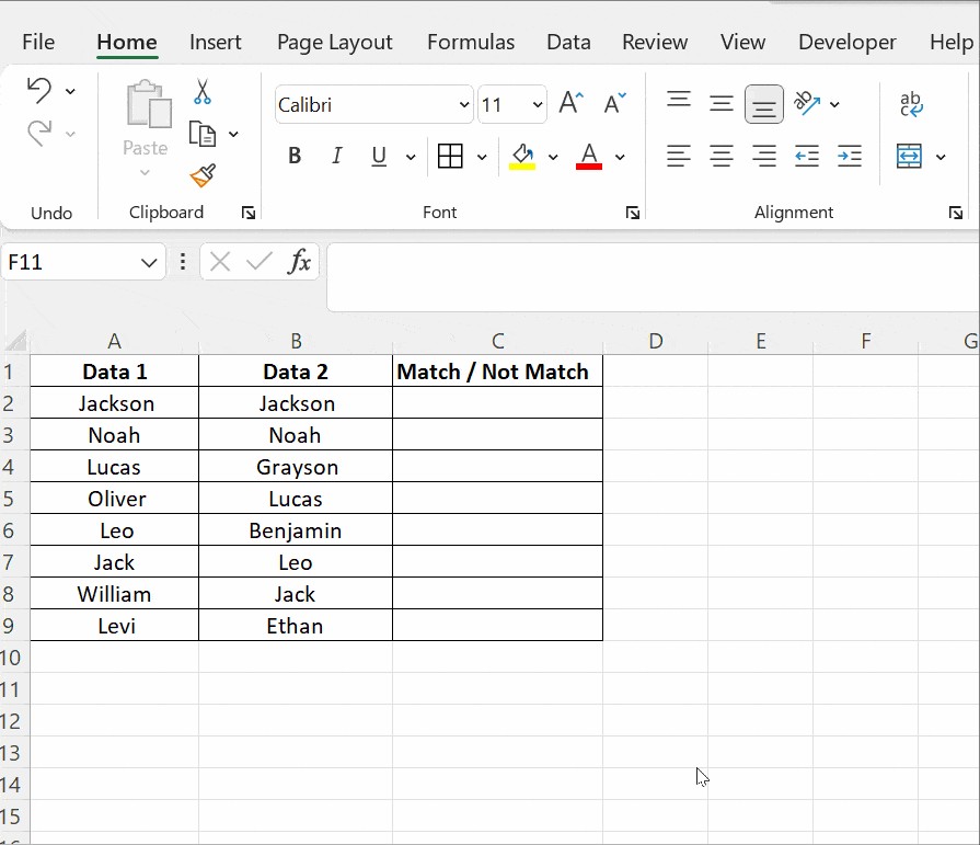
Using the IF Condition for “Match” or “Not Match” Output

While the equals operator provides TRUE/FALSE results, the IF function allows you to display more descriptive text, such as “Match” or “Not Match,” making the comparison results more user-friendly.

Formula: =IF(A2=B2, "Match", "Not Match")

Explanation:

• IF(condition, value_if_true, value_if_false): This is the basic syntax of the IF function.
• A2=B2: This is the condition being tested – whether the value in cell A2 is equal to the value in cell B2.
• "Match": This is the value returned if the condition is TRUE (values match).
• "Not Match": This is the value returned if the condition is FALSE (values do not match).

Steps:

1. Choose a Helper Column: Select an empty column for the comparison results.
2. Enter the Formula: In the first cell of the helper column, enter the formula =IF(A2=B2, "Match", "Not Match").
3. Apply the Formula Down: Drag the fill handle down to apply the formula to all rows.

Example:

You can customize the “Match” and “Not Match” text to suit your needs. For instance, you can use =IF(A2=B2, "Identical", "Different") or even leave the “Not Match” result blank using =IF(A2=B2, "Match", "").

To specifically find mismatches, you can modify the IF formula to highlight differences instead of matches:

Formula for Mismatches: =IF(A2<>B2, "Mismatch", "Match") or =IF(A2<>B2, "Mismatch", "")

Here, <> is the “not equal to” operator. This formula will flag rows where the values in the two columns are different.

Case-Sensitive Comparison with the EXACT() Function

The equals operator and the IF condition are case-insensitive, meaning they treat “Apple” and “apple” as the same. If you need a case-sensitive comparison, use the EXACT() function.

Formula: =EXACT(text1, text2)

Explanation:

• EXACT(text1, text2): This function compares two text strings exactly, including case sensitivity. It returns TRUE if they are identical in case and characters, and FALSE otherwise.

To use EXACT() within an IF condition for “Match” or “Mismatch” results:

Formula: =IF(EXACT(A2, B2), "Match", "Mismatch")

Steps:

1. Choose a Helper Column.
2. Enter the Formula: In the first cell of the helper column, enter =IF(EXACT(A2, B2), "Match", "Mismatch").
3. Apply the Formula Down.

Example:

Column A (Data 1)	Column B (Data 2)	Column C (Case-Sensitive Comparison)
Apple	Apple	Match
apple	Apple	Mismatch
Orange	orange	Mismatch
Banana	Banana	Match

As you can see, EXACT() distinguishes between “Apple” and “apple,” marking them as “Mismatch” because of the case difference.

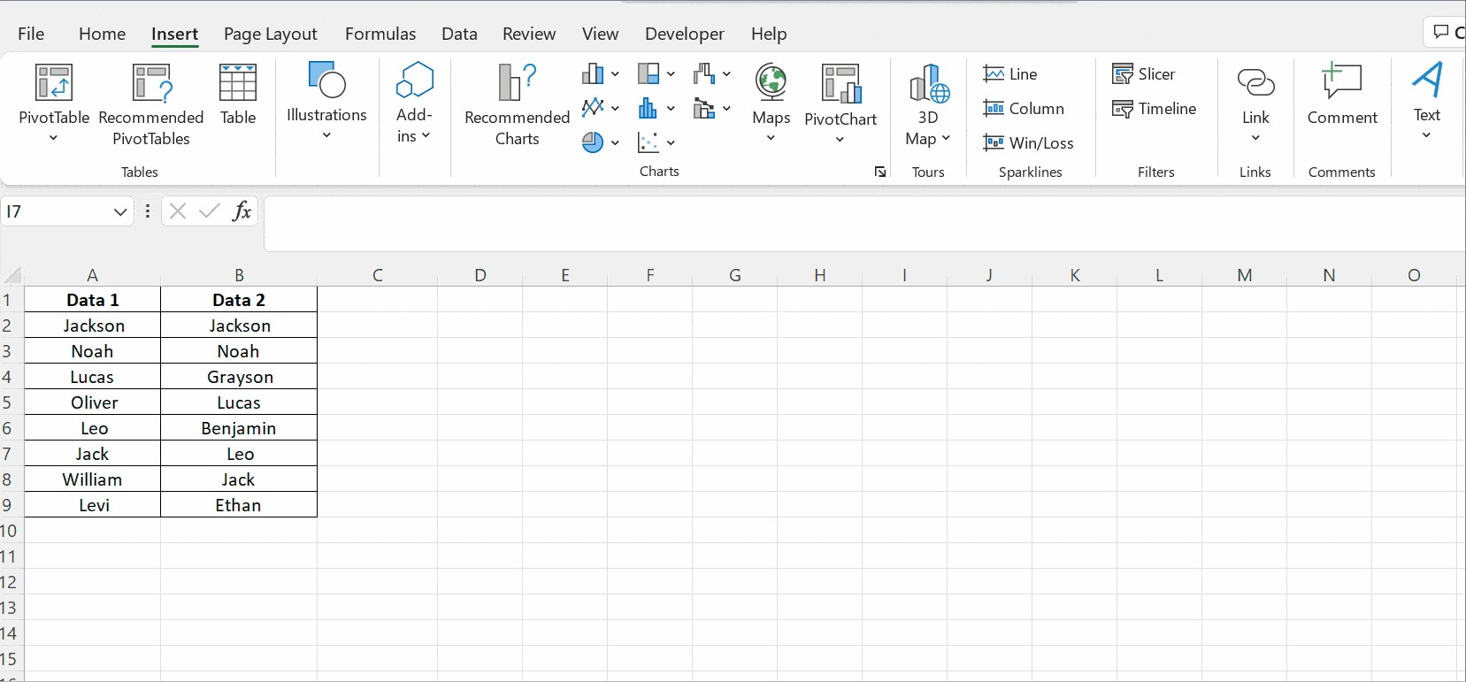
Visual Comparison with Conditional Formatting

Conditional formatting provides a visual way to compare columns by highlighting cells based on certain criteria, such as duplicate or unique values. This method is particularly useful for quickly identifying patterns and differences without adding extra columns.

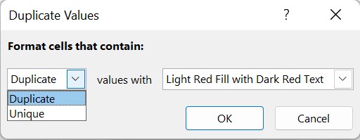
Highlighting Duplicate Values (Values Present in Both Columns):

1. Select the Data Range: Select both columns you want to compare (e.g., columns A and B).
2. Go to Conditional Formatting: On the Home tab, in the Styles group, click Conditional Formatting.
3. Choose Highlight Cells Rules: Select Highlight Cells Rules > Duplicate Values.
4. Customize Formatting: In the “Duplicate Values” dialog box:
   • Ensure “Duplicate” is selected in the dropdown.
   • Choose a formatting style (e.g., Fill with Yellow, Text Color Red). You can also select “Custom Format” for more options.
   • Click OK.

This will highlight values that appear in both selected columns.

Highlighting Unique Values (Values Present in Only One Column):

1. Select the Data Range: Select both columns.
2. Go to Conditional Formatting: Home > Conditional Formatting.
3. Choose Highlight Cells Rules: Select Highlight Cells Rules > Duplicate Values.
4. Change to Unique: In the “Duplicate Values” dialog box, change the dropdown from “Duplicate” to “Unique”.
5. Customize Formatting and Click OK.

This will highlight values that are unique within the selected range, effectively showing values that are present in one column but not the other if you’ve selected both columns.

To clear conditional formatting rules, go to Conditional Formatting > Clear Rules > Clear Rules from Selected Cells or Clear Rules from Entire Sheet.

Conditional formatting is excellent for visual analysis, especially with smaller datasets. For larger spreadsheets or when you need to programmatically process comparison results, formulas or lookup functions might be more suitable.

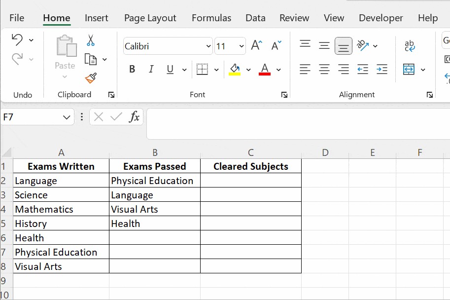
Using VLOOKUP for Advanced Column Comparison

The VLOOKUP function is a powerful tool for comparing columns, especially when you need to check if values from one column exist in another column and potentially retrieve related information.

Scenario: You have a list of items in Column A and another list in Column B. You want to know which items from Column A are also present in Column B.

Formula: =VLOOKUP(A2, $B$2:$B$5, 1, FALSE)

Explanation:

• VLOOKUP(lookup_value, table_array, col_index_num, [range_lookup]) is the syntax of the VLOOKUP function.
• A2: lookup_value – This is the value you are searching for (the value from Column A in the current row).
• $B$2:$B$5: table_array – This is the range in Column B where you are looking for the lookup_value. The $ signs create absolute references, ensuring the range stays fixed when you drag the formula down. Adjust the range B2:B5 to cover your actual data in Column B.
• 1: col_index_num – This specifies which column to return a value from within the table_array. Since we are just checking for presence, we use 1 to return a value from the first (and only, in this case) column of our table_array (Column B).
• FALSE: [range_lookup] – FALSE specifies an exact match. VLOOKUP will only find values in Column B that are exactly the same as the value in A2.

Steps:

1. Choose a Helper Column.
2. Enter the VLOOKUP Formula: In the first cell of the helper column, enter the formula =VLOOKUP(A2, $B$2:$B$5, 1, FALSE). Adjust the table_array range ($B$2:$B$5) to match your Column B data range.
3. Apply the Formula Down.

Example:

Interpreting VLOOKUP Results:

• If VLOOKUP finds a match, it returns the matching value from Column B. In our example, it returns the subject name if the exam taken is also in the list of passed subjects.
• If VLOOKUP does not find a match, it returns #N/A. This indicates that the value from Column A is not present in Column B.

You can combine VLOOKUP with IFERROR to display more user-friendly messages instead of #N/A:

Formula with IFERROR: =IFERROR(VLOOKUP(A2, $B$2:$B$5, 1, FALSE), "Not Found")

IFERROR(value, value_if_error) returns value_if_error if value results in an error; otherwise, it returns the result of value. In this case, if VLOOKUP returns #N/A (error), IFERROR will display “Not Found.” Otherwise, it will display the value returned by VLOOKUP (the matched value from Column B).

Frequently Asked Questions

1. How can I quickly compare two columns in Excel for differences without formulas?

You can use the “Go To Special” feature in Excel to quickly highlight row differences between two columns:

1. Select the Columns: Select both columns you want to compare.
2. Go To Special: Press Ctrl + G (or F5) to open the “Go To” dialog box, and click “Special…”.
3. Choose Row Differences: In the “Go To Special” dialog, select “Row differences” and click “OK”.

Excel will select cells that are different from the corresponding cell in the compared column within each row. Unmatched cells will be highlighted in gray, while matching cells will remain white.

2. How can I compare three or more columns to find rows with matches across all columns?

To check if values in the same row across multiple columns (e.g., columns A, B, and C) are all identical, you can use the AND function within an IF formula:

Formula: =IF(AND(A2=B2, A2=C2), "Full Match", "")

This formula returns “Full Match” only if the values in cells A2, B2, and C2 are all the same. You can extend the AND condition to include more columns as needed (e.g., AND(A2=B2, A2=C2, A2=D2, ...)).

3. Can I use INDEX-MATCH instead of VLOOKUP for comparing columns?

Yes, INDEX-MATCH is a more flexible alternative to VLOOKUP and can also be used for column comparisons. While VLOOKUP requires the lookup column to be the first column in the table array, INDEX-MATCH overcomes this limitation.

For example, to achieve a similar comparison as with VLOOKUP (checking if values from Column D exist in Column A and retrieving corresponding values from Column B if found), you can use:

Formula: =INDEX($B$2:$B$5, MATCH(D2, $A$2:$A$4, 0))

• MATCH(D2, $A$2:$A$4, 0): This part finds the row number in the range $A$2:$A$4 where D2 is found (exact match).
• INDEX($B$2:$B$5, ...): This part uses the row number returned by MATCH to retrieve the corresponding value from the range $B$2:$B$5.

If a match is found, INDEX-MATCH returns the corresponding value from Column B; otherwise, it returns #N/A. You can again use IFERROR to handle #N/A results.

Conclusion

Comparing data in Excel is a vital skill for data analysis and data management. This guide has covered several methods, from simple operators and IF conditions to conditional formatting and lookup functions like VLOOKUP, equipping you with a range of techniques to effectively compare data in Excel columns.

By understanding and applying these methods, you can significantly improve your efficiency and accuracy when working with spreadsheets, enabling you to extract valuable insights and make data-driven decisions with confidence. Experiment with these techniques and choose the methods that best suit your specific data comparison needs in Excel. To further enhance your Excel skills, consider exploring in-depth tutorials on functions like VLOOKUP and other Excel functionalities to become proficient in data manipulation and analysis.