Are you struggling to choose the right statistical test for comparing three groups? COMPARE.EDU.VN offers a comprehensive guide to selecting the appropriate test, ensuring accurate and reliable results. Explore our in-depth analysis and make informed decisions for your research. Statistical Significance, Hypothesis Testing, Data Analysis.
1. Introduction: The Challenge of Comparing Multiple Groups
When conducting research, comparing the means of different groups is a common task. However, when you have more than two groups, the choice of statistical test becomes crucial. Using the wrong test can lead to inaccurate conclusions and potentially flawed research findings. This article provides a detailed overview of the statistical tests suitable for comparing three or more groups, guiding you through the selection process to ensure the integrity of your analysis. Understanding the nuances of each test is essential for drawing valid inferences from your data.
1.1. The Pitfalls of Multiple t-Tests
A common mistake researchers make when comparing three or more groups is performing multiple independent t-tests. For example, if you have three groups (A, B, and C) and you want to compare their means, you might be tempted to conduct three separate t-tests: A vs. B, A vs. C, and B vs. C. While this approach might seem straightforward, it significantly inflates the probability of making a Type I error, also known as a false positive. A Type I error occurs when you reject the null hypothesis (i.e., conclude there is a significant difference between the groups) when the null hypothesis is actually true (i.e., there is no real difference between the groups).
Each t-test has a predetermined alpha level (α), which is the probability of making a Type I error. Typically, the alpha level is set at 0.05, meaning there is a 5% chance of incorrectly rejecting the null hypothesis. When you perform multiple t-tests, the overall probability of making at least one Type I error increases substantially. For k independent comparisons, the overall error rate is calculated as 1 – (1 – α)^k. For instance, with three t-tests and an alpha level of 0.05, the overall error rate becomes 1 – (1 – 0.05)^3 = 0.1426, or 14.26%. This is much higher than the intended 5% and makes the results unreliable.
1.2. The Solution: Analysis of Variance (ANOVA)
To avoid the inflated error rate associated with multiple t-tests, the appropriate method for comparing the means of three or more groups is Analysis of Variance (ANOVA). ANOVA is a statistical test that assesses whether there are any statistically significant differences between the means of two or more independent groups. Unlike t-tests, ANOVA performs a single, overall test that controls for the Type I error rate, maintaining the desired alpha level (typically 0.05).
ANOVA works by partitioning the total variability in the data into different sources: the variability between groups (i.e., the variance among the group means) and the variability within groups (i.e., the variance within each group). By comparing these two sources of variability, ANOVA determines whether the differences between the group means are larger than what would be expected by chance. If the between-group variance is significantly larger than the within-group variance, it suggests that there are real differences between the group means.
1.3. When to Use ANOVA
ANOVA is most appropriate when you have:
- Three or more independent groups: ANOVA is designed to compare the means of multiple groups simultaneously.
- A continuous dependent variable: The variable you are measuring must be continuous (e.g., height, weight, test score).
- Independent observations: The data points in each group should be independent of each other.
- Normally distributed data: The data in each group should be approximately normally distributed.
- Homogeneity of variances: The variances of the groups should be roughly equal.
If your data violate the assumptions of normality or homogeneity of variances, there are alternative non-parametric tests you can use, which will be discussed later in this article.
2. Understanding One-Way ANOVA
One-way ANOVA is the most basic type of ANOVA and is used when you have one independent variable (factor) with three or more levels (groups) and one continuous dependent variable. The goal of one-way ANOVA is to determine whether there are any statistically significant differences between the means of the groups.
2.1. The Logic Behind ANOVA: Variance Decomposition
The core principle of ANOVA is to decompose the total variance in the data into different components. This allows us to assess the relative contributions of the between-group variability and the within-group variability.
- Total Variance (SST): This represents the total variability in the data, regardless of group membership. It is calculated as the sum of the squared differences between each individual data point and the overall mean (grand mean).
- Between-Group Variance (SSB): This represents the variability between the group means. It is calculated as the sum of the squared differences between each group mean and the grand mean, weighted by the sample size of each group.
- Within-Group Variance (SSW): This represents the variability within each group. It is calculated as the sum of the squared differences between each individual data point and its respective group mean.
The fundamental equation of ANOVA is:
SST = SSB + SSW
This equation states that the total variance is equal to the sum of the between-group variance and the within-group variance.
2.2. Calculating the F-Statistic
The F-statistic is the test statistic used in ANOVA to determine whether there are significant differences between the group means. It is calculated as the ratio of the between-group variance to the within-group variance:
F = MSB / MSW
Where:
- MSB (Mean Square Between): This is the between-group variance divided by its degrees of freedom (number of groups – 1).
- MSW (Mean Square Within): This is the within-group variance divided by its degrees of freedom (total sample size – number of groups).
A large F-statistic indicates that the between-group variance is much larger than the within-group variance, suggesting that there are significant differences between the group means.
2.3. Interpreting the Results
To determine whether the F-statistic is statistically significant, it is compared to a critical value from the F-distribution. The F-distribution is a probability distribution that depends on the degrees of freedom for the between-group variance and the within-group variance.
If the calculated F-statistic is greater than the critical value from the F-distribution, we reject the null hypothesis and conclude that there are statistically significant differences between the means of the groups. The p-value associated with the F-statistic indicates the probability of observing an F-statistic as large as, or larger than, the one calculated from the data, assuming the null hypothesis is true. A small p-value (typically less than 0.05) provides strong evidence against the null hypothesis.
2.4. Example of One-Way ANOVA
Imagine a researcher wants to compare the effectiveness of three different teaching methods on student test scores. The researcher randomly assigns students to one of three groups:
- Group A: Traditional lecture-based teaching.
- Group B: Interactive, group-based learning.
- Group C: Online, self-paced learning.
After a semester, all students take the same standardized test. The researcher uses one-way ANOVA to analyze the test scores.
- Null Hypothesis: There is no difference in mean test scores between the three teaching methods.
- Alternative Hypothesis: There is a difference in mean test scores between the three teaching methods.
The ANOVA results show an F-statistic of 4.5 and a p-value of 0.015. Since the p-value is less than 0.05, the researcher rejects the null hypothesis and concludes that there is a statistically significant difference in mean test scores between the three teaching methods.
2.5. Illustration of Between-Group and Within-Group Variance
To further illustrate the concept of between-group and within-group variance, consider the following scenario. Suppose we are comparing the heights of people from three different countries: Country X, Country Y, and Country Z.
Figure 1: Height distribution across three countries with similar between-group variance but different within-group variances.
Scenario 1: Small Within-Group Variance
If the heights of people within each country are very similar (i.e., small within-group variance), even small differences in the average heights between the countries (i.e., between-group variance) may be statistically significant. This is because the small within-group variance makes it easier to detect the differences between the group means.
Scenario 2: Large Within-Group Variance
If the heights of people within each country are highly variable (i.e., large within-group variance), larger differences in the average heights between the countries are needed to achieve statistical significance. This is because the large within-group variance makes it more difficult to distinguish the differences between the group means from the random variability within each group.
This example highlights the importance of considering both the between-group variance and the within-group variance when interpreting the results of ANOVA.
3. Post-Hoc Tests: Delving Deeper into Group Differences
If the one-way ANOVA reveals a statistically significant difference between the group means, it indicates that not all group means are equal. However, ANOVA does not tell you which specific groups differ from each other. To identify these specific differences, you need to perform post-hoc tests.
Post-hoc tests are pairwise comparisons that are conducted after a significant ANOVA result to determine which groups differ significantly from each other. These tests adjust the alpha level to account for the multiple comparisons, controlling for the overall Type I error rate.
3.1. Common Post-Hoc Tests
Several post-hoc tests are available, each with its own strengths and weaknesses. Some of the most commonly used post-hoc tests include:
- Tukey’s Honestly Significant Difference (HSD): This test is widely used and provides good control over the Type I error rate. It is generally recommended when you have equal sample sizes in each group.
- Bonferroni Correction: This is a simple and conservative method that adjusts the alpha level by dividing it by the number of comparisons. While it is easy to implement, it can be overly conservative, especially when you have a large number of groups.
- Scheffé’s Method: This is another conservative method that is suitable for both pairwise comparisons and more complex contrasts. It is often used when you have unequal sample sizes and want to perform a variety of different comparisons.
- Fisher’s Least Significant Difference (LSD): This is the least conservative post-hoc test and has the highest risk of Type I errors. It is generally not recommended unless you have a strong justification for using it.
- Dunnett’s Test: This test is used when you have a control group and want to compare each of the other groups to the control group.
3.2. Choosing the Right Post-Hoc Test
The choice of post-hoc test depends on the specific research question, the sample sizes of the groups, and the desired level of control over the Type I error rate.
- If you have equal sample sizes and want to compare all possible pairs of groups, Tukey’s HSD is a good choice.
- If you have unequal sample sizes and want to perform a variety of different comparisons, Scheffé’s method may be more appropriate.
- If you have a control group and want to compare each of the other groups to the control group, Dunnett’s test is the most suitable option.
- If you want a simple and conservative method, the Bonferroni correction can be used, but be aware that it may be overly conservative.
3.3. Example of Post-Hoc Tests
Referring back to the example of the researcher comparing three different teaching methods, suppose the one-way ANOVA revealed a significant difference in mean test scores between the groups. To determine which specific teaching methods differed from each other, the researcher performs Tukey’s HSD post-hoc test.
The results of Tukey’s HSD show that:
- Group B (interactive, group-based learning) had significantly higher test scores than Group A (traditional lecture-based teaching).
- Group C (online, self-paced learning) had significantly higher test scores than Group A (traditional lecture-based teaching).
- There was no significant difference in test scores between Group B and Group C.
Based on these results, the researcher concludes that both interactive, group-based learning and online, self-paced learning are more effective than traditional lecture-based teaching in improving student test scores.
3.4. Reporting Post-Hoc Test Results
When reporting the results of post-hoc tests, it is important to include the following information:
- The specific post-hoc test that was used (e.g., Tukey’s HSD, Bonferroni correction).
- The p-values for each pairwise comparison.
- A clear statement of which groups differed significantly from each other.
You can also use letters to indicate which groups are significantly different. For example, you could assign the letter “A” to the group with the highest mean, the letter “B” to the group with the second-highest mean, and so on. Groups with the same letter are not significantly different from each other.
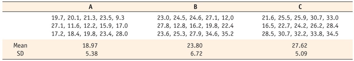
Table 1: Comparative mean bond strength according to different types of resin with ANOVA results.
For example, if Group A and Group C have the letter “A” and Group B has the letter “B,” this indicates that Group B is significantly different from both Group A and Group C, but Group A and Group C are not significantly different from each other.
4. Two-Way ANOVA: Exploring Multiple Factors
While one-way ANOVA is used to compare the means of groups based on a single factor, two-way ANOVA is used when you have two independent variables (factors) and want to examine their individual and combined effects on a continuous dependent variable.
4.1. Understanding Main Effects and Interaction Effects
In two-way ANOVA, you are interested in two types of effects:
- Main Effects: The main effect of a factor is the effect of that factor on the dependent variable, regardless of the levels of the other factor.
- Interaction Effects: An interaction effect occurs when the effect of one factor on the dependent variable depends on the levels of the other factor.
For example, suppose you are studying the effects of two factors on plant growth: fertilizer type (Factor A) and watering frequency (Factor B). The main effect of fertilizer type would be the effect of fertilizer type on plant growth, regardless of the watering frequency. The main effect of watering frequency would be the effect of watering frequency on plant growth, regardless of the fertilizer type.
An interaction effect would occur if the effect of fertilizer type on plant growth depends on the watering frequency. For example, one type of fertilizer might be more effective when used with frequent watering, while another type of fertilizer might be more effective when used with infrequent watering.
4.2. Assumptions of Two-Way ANOVA
Two-way ANOVA has the same assumptions as one-way ANOVA:
- A continuous dependent variable.
- Independent observations.
- Normally distributed data within each group.
- Homogeneity of variances across all groups.
Additionally, two-way ANOVA assumes that there is no correlation between the two factors.
4.3. Example of Two-Way ANOVA
A researcher wants to investigate the effects of two factors on employee productivity: training program (Factor A: New Program vs. Old Program) and work environment (Factor B: Open Office vs. Private Office). The researcher randomly assigns employees to one of four groups:
- Group 1: New Program, Open Office
- Group 2: New Program, Private Office
- Group 3: Old Program, Open Office
- Group 4: Old Program, Private Office
After a month, the researcher measures the productivity of each employee. The researcher uses two-way ANOVA to analyze the data.
The results of the two-way ANOVA show:
- A significant main effect of training program (p < 0.05): Employees in the New Program group had significantly higher productivity than employees in the Old Program group.
- A significant main effect of work environment (p < 0.05): Employees in the Private Office group had significantly higher productivity than employees in the Open Office group.
- A significant interaction effect between training program and work environment (p < 0.05): The effect of the training program on productivity depended on the work environment. Specifically, the New Program was much more effective in the Private Office environment than in the Open Office environment.
Based on these results, the researcher concludes that both the training program and the work environment have a significant impact on employee productivity. Furthermore, the interaction effect suggests that the effectiveness of the training program is influenced by the type of work environment.
4.4. Interpreting Interaction Effects
When a significant interaction effect is present, it is crucial to interpret it carefully. An interaction effect indicates that the relationship between one factor and the dependent variable changes depending on the level of the other factor.
To understand the nature of the interaction effect, it is helpful to create a graph that displays the mean values of the dependent variable for each combination of the two factors. This graph can help you visualize how the effect of one factor changes across the levels of the other factor.
In the example above, a graph of employee productivity for each combination of training program and work environment would show that the New Program leads to higher productivity in the Private Office environment, but has a smaller impact in the Open Office environment. This visualization would help to clarify the nature of the interaction effect.
5. Non-Parametric Alternatives to ANOVA
If your data violate the assumptions of normality or homogeneity of variances, ANOVA may not be the most appropriate test. In these cases, non-parametric alternatives to ANOVA can be used. Non-parametric tests do not rely on the assumption of normality and are therefore more robust to violations of this assumption.
5.1. Kruskal-Wallis Test
The Kruskal-Wallis test is a non-parametric alternative to one-way ANOVA. It is used to compare the medians of three or more independent groups. The Kruskal-Wallis test is based on ranks, rather than the actual data values. This makes it less sensitive to outliers and violations of normality.
When to Use Kruskal-Wallis:
- You have three or more independent groups.
- Your dependent variable is continuous or ordinal.
- Your data do not meet the assumptions of normality or homogeneity of variances.
Example:
A researcher wants to compare the customer satisfaction ratings (on a scale of 1 to 10) for three different brands of smartphones. The data are not normally distributed. The researcher uses the Kruskal-Wallis test to compare the medians of the satisfaction ratings for the three brands.
5.2. Friedman Test
The Friedman test is a non-parametric alternative to repeated measures ANOVA. It is used to compare the medians of three or more related groups. The Friedman test is also based on ranks and is suitable when you have repeated measurements on the same subjects or matched groups.
When to Use Friedman Test:
- You have three or more related groups (repeated measures or matched groups).
- Your dependent variable is continuous or ordinal.
- Your data do not meet the assumptions of normality or homogeneity of variances.
Example:
A researcher wants to compare the pain levels of patients after three different treatments. The pain levels are measured on a scale of 1 to 10. The data are not normally distributed. The researcher uses the Friedman test to compare the medians of the pain levels for the three treatments.
5.3. Post-Hoc Tests for Non-Parametric Tests
If the Kruskal-Wallis or Friedman test reveals a significant difference between the groups, you can perform post-hoc tests to determine which specific groups differ from each other. Several post-hoc tests are available for non-parametric tests, such as the Dunn’s test for Kruskal-Wallis and the Wilcoxon signed-rank test with Bonferroni correction for Friedman test.
5.4. Choosing Between Parametric and Non-Parametric Tests
The decision of whether to use a parametric test (such as ANOVA) or a non-parametric test (such as Kruskal-Wallis or Friedman) depends on the characteristics of your data and the assumptions of the tests.
- If your data meet the assumptions of normality and homogeneity of variances, ANOVA is generally the preferred choice because it is more powerful than non-parametric tests.
- If your data violate the assumptions of normality or homogeneity of variances, a non-parametric test is more appropriate.
It is always a good practice to examine your data carefully and consider the assumptions of the statistical tests before making a decision.
6. Reporting ANOVA Results
When reporting the results of ANOVA, it is important to provide all the necessary information to allow readers to understand your analysis and interpret your findings.
6.1. Essential Information to Include
The following information should be included in your report:
- A clear statement of the research question and hypotheses.
- A description of the study design and the participants.
- A description of the variables that were measured and how they were measured.
- A statement of whether the assumptions of ANOVA were met.
- The F-statistic, degrees of freedom, and p-value for the overall ANOVA test.
- If the overall ANOVA test was significant, the results of the post-hoc tests, including the specific post-hoc test that was used, the p-values for each pairwise comparison, and a clear statement of which groups differed significantly from each other.
- A table or graph summarizing the results.
- A discussion of the implications of the findings.
6.2. Example of Reporting ANOVA Results
“A one-way ANOVA was conducted to compare the effectiveness of three different teaching methods on student test scores. The independent variable was teaching method (traditional lecture-based, interactive group-based, and online self-paced), and the dependent variable was student test score. The assumptions of normality and homogeneity of variances were met. The results of the ANOVA showed a significant effect of teaching method on student test scores, F(2, 97) = 4.5, p = 0.015. Post-hoc comparisons using Tukey’s HSD revealed that the interactive group-based teaching method resulted in significantly higher test scores than the traditional lecture-based teaching method (p = 0.025), and the online self-paced teaching method resulted in significantly higher test scores than the traditional lecture-based teaching method (p = 0.032). There was no significant difference in test scores between the interactive group-based teaching method and the online self-paced teaching method (p = 0.951).”
6.3. Using Tables and Graphs
Tables and graphs can be very helpful in summarizing and presenting the results of ANOVA. A table can be used to display the means and standard deviations for each group, as well as the results of the post-hoc tests. A graph, such as a bar chart or a box plot, can be used to visually represent the differences between the group means.
Ensure that your tables and graphs are clearly labeled and easy to understand. Use appropriate axis labels, legends, and titles.
6.4. Discussing the Implications of the Findings
In the discussion section of your report, you should interpret your findings in the context of your research question and hypotheses. Discuss the implications of your findings for theory and practice. Consider the limitations of your study and suggest directions for future research.
For example, in the teaching method example, you might discuss the implications of the findings for educators and suggest that they consider incorporating interactive group-based learning and online self-paced learning into their teaching practices. You might also acknowledge the limitations of the study, such as the fact that it was conducted in a single school district, and suggest that future research should examine the effectiveness of these teaching methods in other settings.
7. Using Statistical Software Packages
Performing ANOVA and post-hoc tests by hand can be tedious and time-consuming. Fortunately, several statistical software packages are available that can automate these calculations.
7.1. Popular Statistical Software Packages
Some of the most popular statistical software packages include:
- SPSS (Statistical Package for the Social Sciences): SPSS is a widely used statistical software package that offers a comprehensive set of tools for data analysis, including ANOVA and post-hoc tests.
Figure 2: SPSS statistical package interface.
- R: R is a free and open-source statistical software environment that is widely used in academia and industry. R offers a vast array of packages for data analysis, including ANOVA and post-hoc tests.
- SAS (Statistical Analysis System): SAS is a powerful statistical software package that is commonly used in business and government. SAS offers a comprehensive set of tools for data analysis, including ANOVA and post-hoc tests.
- Stata: Stata is a statistical software package that is commonly used in economics, sociology, and other social sciences. Stata offers a comprehensive set of tools for data analysis, including ANOVA and post-hoc tests.
7.2. Steps for Performing ANOVA in SPSS
To perform ANOVA in SPSS, follow these steps:
- Enter your data into SPSS.
- Go to Analyze > Compare Means > One-Way ANOVA.
- Select your dependent variable and independent variable.
- Click on Post Hoc and select the post-hoc test you want to use.
- Click OK to run the analysis.
SPSS will generate a table of results, including the F-statistic, degrees of freedom, p-value, and the results of the post-hoc tests.
7.3. Tips for Using Statistical Software
- Familiarize yourself with the software’s documentation and tutorials.
- Double-check your data entry to ensure accuracy.
- Carefully select the appropriate options and settings for your analysis.
- Interpret the results cautiously and in the context of your research question.
- Consult with a statistician if you have any questions or concerns.
8. Conclusion: Making Informed Decisions
Choosing the right statistical test for comparing three or more groups is crucial for ensuring the accuracy and validity of your research findings. ANOVA is the appropriate method when you have three or more independent groups, a continuous dependent variable, and your data meet the assumptions of normality and homogeneity of variances. Post-hoc tests are used to determine which specific groups differ from each other. If your data violate the assumptions of ANOVA, non-parametric alternatives, such as the Kruskal-Wallis test and the Friedman test, can be used.
By understanding the principles of ANOVA, post-hoc tests, and non-parametric alternatives, you can make informed decisions about which statistical test is most appropriate for your research question and data. This will help you to draw valid conclusions from your data and contribute to the body of knowledge in your field.
Are you looking for more detailed comparisons and objective insights to guide your decisions? Visit COMPARE.EDU.VN today! Located at 333 Comparison Plaza, Choice City, CA 90210, United States. Contact us via Whatsapp: +1 (626) 555-9090. Our website COMPARE.EDU.VN provides comprehensive comparisons to help you make smarter choices.
9. Frequently Asked Questions (FAQ)
1. What is ANOVA and when should I use it?
ANOVA (Analysis of Variance) is a statistical test used to compare the means of two or more groups. It should be used when you have a continuous dependent variable and a categorical independent variable with three or more levels (groups).
2. What is the difference between one-way ANOVA and two-way ANOVA?
One-way ANOVA is used when you have one independent variable (factor) with three or more levels, while two-way ANOVA is used when you have two independent variables (factors) and want to examine their individual and combined effects on a continuous dependent variable.
3. What are post-hoc tests and why are they necessary?
Post-hoc tests are pairwise comparisons that are conducted after a significant ANOVA result to determine which specific groups differ significantly from each other. They are necessary because ANOVA only tells you that there is a difference between the groups, but not which groups are different.
4. What are some common post-hoc tests?
Some common post-hoc tests include Tukey’s HSD, Bonferroni correction, Scheffé’s method, Fisher’s LSD, and Dunnett’s test.
5. What do I do if my data violate the assumptions of ANOVA?
If your data violate the assumptions of normality or homogeneity of variances, you can use non-parametric alternatives to ANOVA, such as the Kruskal-Wallis test or the Friedman test.
6. What is the Kruskal-Wallis test and when should I use it?
The Kruskal-Wallis test is a non-parametric alternative to one-way ANOVA. It is used to compare the medians of three or more independent groups when your data do not meet the assumptions of normality or homogeneity of variances.
7. What is the Friedman test and when should I use it?
The Friedman test is a non-parametric alternative to repeated measures ANOVA. It is used to compare the medians of three or more related groups when your data do not meet the assumptions of normality or homogeneity of variances.
8. How do I report the results of ANOVA?
When reporting the results of ANOVA, you should include a clear statement of the research question and hypotheses, a description of the study design and participants, a description of the variables that were measured, a statement of whether the assumptions of ANOVA were met, the F-statistic, degrees of freedom, p-value, and the results of the post-hoc tests.
9. Can I use t-tests instead of ANOVA to compare three or more groups?
No, you should not use t-tests instead of ANOVA to compare three or more groups. Performing multiple t-tests inflates the probability of making a Type I error, leading to inaccurate conclusions. ANOVA is the appropriate method for comparing the means of three or more groups.
10. Where can I find more information about ANOVA and other statistical tests?
You can find more information about ANOVA and other statistical tests on the compare.edu.vn website, in textbooks on statistics, and from online resources such as statistical tutorials and videos.