What Excel Formula To Use To Compare Two Columns

What Excel Formula To Use To Compare Two Columns? COMPARE.EDU.VN provides a comprehensive guide that simplifies data comparison in Excel, offering you the knowledge and skills to efficiently analyze your data. With the right formulas, you can unlock valuable insights, improve accuracy, and save time when working with spreadsheets. Discover the power of Excel with COMPARE.EDU.VN to analyze data, identify matches and differences.

1. Why Comparing Two Columns in Excel Is Essential

Excel is more than just a spreadsheet program; it’s a powerful tool for data storage, manipulation, and informed decision-making. Data analysts rely on Excel to gather crucial information that drives marketing and sales strategies.

When a cell lacks information, it can significantly impact analyses, especially when dealing with large, interconnected spreadsheets. Comparing two columns within the same or different spreadsheets becomes essential for data analysts. Manual comparison is tedious and time-consuming. The ability to quickly identify whether a cell contains data or not is crucial.

Excel offers various ways to compare data, presenting results as TRUE/FALSE, Match/Not Match, or custom user-defined messages, streamlining the data analysis workflow and empowering you to draw meaningful conclusions. This makes it essential to master what excel formula to use to compare two columns.

2. Methods to Compare Two Columns in Excel

Depending on the task, there are many ways to compare two columns in Excel. Each method has its advantages. Here are some common techniques:

• Highlighting unique or duplicate values using functions.
• Displaying unique or duplicate values using conditional formatting or formulas.
• Performing row-by-row comparisons.
• Utilizing LOOKUP formulas.

Choosing the right approach depends on your specific needs and the desired outcome of the comparison.

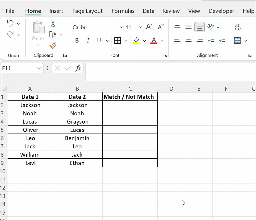
3. Comparing Two Columns Using the Equals Operator

A basic yet effective method to compare two columns is using the equals operator (=) for a row-by-row comparison. This allows you to quickly identify matching data, with the results displayed as “Match” or “Not Match,” or TRUE/FALSE values.

For example, the formula =A2=B2 checks if the values in cell A2 match the value in cell B2. The result will be TRUE if they match and FALSE if they don’t.

To implement this, enter the formula in the first cell where you want the result (e.g., C2) and then drag the fill handle (the small square at the bottom-right of the cell) down to apply the formula to the rest of the rows. This is the basic what excel formula to use to compare two columns.

4. Leveraging the IF Condition for Column Comparison

The IF condition in Excel allows for more customized comparisons. You can specify what result to display if the values match and what to display if they don’t.

4.1. Identifying Matching Values

The formula =IF(A2=B2,”Match”,””) compares the values in cells A2 and B2. If they match, the formula returns “Match.” Otherwise, it leaves the cell blank. This is the simplest what excel formula to use to compare two columns.

4.2. Identifying Mismatching Values

To identify mismatching values, you can modify the formula to =IF(A2=B2,”Match”,”Not a Match”). This formula will return “Match” if the values are the same and “Not a Match” if they are different.

4.3. Comparing for Differences

To specifically compare two columns for differences, use the non-equality operator (<>). The formula =IF(A2<>B2,”Match”,”Not a Match”) will return “Match” if the values are different and “Not a Match” if they are the same.

5. Using the EXACT() Function for Case-Sensitive Comparisons

When you need a case-sensitive comparison, the EXACT() function is invaluable. The EXACT() function compares two text strings and returns TRUE if they are exactly the same, including case, and FALSE otherwise.

5.1. Syntax and Usage

The syntax for the EXACT() function is =EXACT(text1, text2), where text1 and text2 are the two text strings you want to compare.

5.2. Example

Suppose you have “Nova Scotia” in cell A2 and “nova scotia” in cell B2. The formula =IF(A2=B2,”Match”,”Mismatch”) will return “Match” because the equals operator is case-insensitive.

However, the formula =IF(EXACT(A2,B2),”Match”,”Mismatch”) will return “Mismatch” because the EXACT() function is case-sensitive and recognizes that the capitalization is different.

5.3. How EXACT() Works

The EXACT() function performs an exact comparison and returns TRUE or FALSE. The IF condition then uses this result to determine which message to display, making it a powerful tool for precise data comparison.

6. Conditional Formatting for Visual Comparisons

Conditional formatting allows you to visually highlight cells based on certain criteria. This is useful for quickly identifying duplicate or unique values in two columns.

6.1. Highlighting Duplicate Values

To highlight duplicate values, select both columns, then go to Home → Conditional Formatting → Highlight Cells Rules → Duplicate Values. In the dialog box, choose “Duplicate” from the dropdown menu and select the formatting style you want to apply (e.g., fill with red color).

This will highlight all cells containing values that appear in both columns, providing a visual representation of matching data.

6.2. Highlighting Unique Values

To highlight unique values, follow the same steps as above, but choose “Unique” from the dropdown menu. This will highlight all cells containing values that appear only in one of the columns, making it easy to identify differences.

6.3. Clearing Conditional Formatting

To remove conditional formatting, go to Conditional Formatting → Clear Rules → Clear Rules from Selected Cells.

6.4. Advantages of Conditional Formatting

Conditional formatting is ideal when you want to quickly visualize matches or differences without adding a third column. It’s suitable for smaller tables where a visual overview is sufficient.

7. Utilizing Lookup Functions for Advanced Comparisons

Lookup functions, such as VLOOKUP, HLOOKUP, and XLOOKUP, are powerful tools for comparing data across columns and tables. They allow you to search for a value in one column and return a corresponding value from another column.

7.1. VLOOKUP for Vertical Lookup

VLOOKUP (Vertical Lookup) searches for a value in the first column of a range and returns a value from a specified column in the same row.

Syntax

The syntax for VLOOKUP is =VLOOKUP(lookup_value, table_array, col_index_num, [range_lookup])

• lookup_value: The value you want to search for.
• table_array: The range of cells where you want to search.
• col_index_num: The column number in the table_array from which to return a value.
• range_lookup: A logical value (TRUE or FALSE) that specifies whether to find an approximate or exact match.

Example

Suppose you have a list of exams taken by a student in column A and a list of subjects the student passed in column B. You want to determine which exams the student has cleared.

In cell C2, enter the formula =VLOOKUP(A2,$B$2:$B$5,1,FALSE). This formula searches for the value in A2 within the range B2:B5. If it finds a match, it returns the value from the first column (column B) of the range. If it doesn’t find a match, it returns #N/A.

The $ symbols in $B$2:$B$5 create an absolute reference, which ensures that the range remains fixed when you drag the formula down to apply it to other cells.

7.2. How VLOOKUP Works

• VLOOKUP(A2,..,..,..): Takes the value in cell A2 as the lookup value.
• VLOOKUP(A2,$B$2:$B$5,..,..): Compares the lookup value with the values in the range B2:B5.
• VLOOKUP(A2,$B$2:$B$5,1,..): Specifies that the value should be returned from the first column of the range.
• VLOOKUP(A2,$B$2:$B$5,1,FALSE): Ensures that only exact matches are considered.

By dragging the formula down, you can quickly identify which subjects have been cleared and which have not, indicated by #N/A.

8. Combining IF with AND/OR for Complex Criteria

For more complex comparisons, you can combine the IF condition with the AND and OR functions.

8.1. Using AND

The AND function checks if all conditions are true. For example, to find rows where all cells have the same values in columns A, B, and C, use the formula =IF(AND(A2=B2,A2=C2),”Full match”,””). This formula returns “Full match” only if the values in A2, B2, and C2 are identical.

8.2. Using OR

The OR function checks if at least one condition is true. To find rows where any two cells have the same values in columns A, B, and C, use the formula =IF(OR(A2=B2,B2=C2,A2=C2),”Match”,””). This formula returns “Match” if any two of the cells A2, B2, or C2 have the same value.

9. INDEX-MATCH as an Alternative to VLOOKUP

The INDEX-MATCH function is a flexible alternative to VLOOKUP, especially when you need to match columns in different tables and pull matching entries.

9.1. Syntax and Usage

The INDEX function returns the value of a cell within a range, and the MATCH function finds the position of a value within a range.

The basic syntax is =INDEX(return_range, MATCH(lookup_value, lookup_range, 0))

• return_range: The range from which to return the value.
• lookup_value: The value to search for.
• lookup_range: The range in which to search for the lookup_value.
• 0: Specifies an exact match.

9.2. Example

Suppose you have a list of IDs in column A and corresponding names in column B. In column D, you have another list of IDs, and you want to find the names corresponding to those IDs from the first table.

In cell E2, enter the formula =INDEX($B$2:$B$4,MATCH(D2,$A$2:$A$4,0)). This formula searches for the value in D2 within the range A2:A4. If it finds a match, it returns the corresponding name from the range B2:B4. If it doesn’t find a match, it returns #N/A.

10. Addressing Common Challenges and Errors

When comparing columns in Excel, you might encounter certain challenges and errors.

10.1. Handling #N/A Errors

The #N/A error typically occurs when a lookup function cannot find a match. To handle this error, you can use the IFERROR function.

For example, instead of =VLOOKUP(A2,$B$2:$B$5,1,FALSE), use =IFERROR(VLOOKUP(A2,$B$2:$B$5,1,FALSE),”Not Found”). This formula will return “Not Found” if VLOOKUP returns #N/A.

10.2. Dealing with Case Sensitivity

If you need a case-sensitive comparison, remember to use the EXACT() function, as the standard equals operator (=) is case-insensitive.

10.3. Ensuring Data Consistency

Make sure that the data in both columns is consistent in terms of formatting and data types. Inconsistent data can lead to incorrect comparisons.

11. Optimizing Performance for Large Datasets

When working with large datasets, performance can be a concern. Here are some tips to optimize performance:

• Use helper columns: Instead of complex formulas, break them down into smaller, simpler formulas in helper columns.
• Avoid volatile functions: Functions like NOW() and TODAY() recalculate every time the worksheet changes, which can slow down performance.
• Use array formulas sparingly: Array formulas can be powerful, but they can also be computationally intensive.
• Ensure efficient formulas: Using techniques such as using INDEX/MATCH instead of VLOOKUP can improve efficiency because INDEX/MATCH doesn’t need to read the entire table.

12. Step-by-Step Guide: Comparing Two Columns for Email Addresses

Comparing two columns for email addresses requires precise matching. Here’s a step-by-step guide:

1. Open Excel: Open the Excel spreadsheet containing the email address columns you want to compare.
2. Select the First Cell: Select the first cell in the column where you want the comparison result to appear (e.g., C2).
3. Enter the Formula:
   • For a case-insensitive comparison, enter =IF(A2=B2, "Match", "No Match").
   • For a case-sensitive comparison, enter =IF(EXACT(A2, B2), "Match", "No Match").
4. Apply the Formula: Drag the fill handle (the small square at the bottom-right of cell C2) down to apply the formula to all the rows in the columns.
5. Review the Results: Review the “Match” and “No Match” results in column C to identify identical and different email addresses.
6. Conditional Formatting (Optional): To highlight matches or differences, select all the result cells in column C, go to Conditional Formatting, and set rules to format cells containing “Match” or “No Match.”

13. Step-by-Step Guide: Comparing Two Columns for Phone Numbers

Phone numbers often include variations in formatting (spaces, hyphens, parentheses), so standardization is important. Here’s how:

1. Standardize Phone Numbers: Use the SUBSTITUTE function to remove spaces, hyphens, and parentheses. For example, if phone numbers are in column A, use =SUBSTITUTE(SUBSTITUTE(SUBSTITUTE(A2," ",""),"-",""),"(","") in column D to clean the data. Repeat for column B, placing cleaned numbers in column E.
2. Compare Standardized Numbers: In column F, use the formula =IF(D2=E2, "Match", "No Match") to compare the cleaned phone numbers.
3. Apply and Review: Drag the formula down to apply it to all rows. Review the results to identify matching and non-matching phone numbers.
4. Conditional Formatting (Optional): Highlight matches or differences using conditional formatting for a visual overview.

14. Tips for Effective Column Comparison

• Understand Your Data: Know the type of data you’re working with and whether case sensitivity is important.
• Choose the Right Method: Select the comparison method that best suits your needs, whether it’s a simple equals operator, conditional formatting, or a more advanced lookup function.
• Use Absolute References: When using formulas that refer to a specific range, use absolute references ($) to prevent the range from changing when you drag the formula.
• Test Your Formulas: Always test your formulas on a small sample of data to ensure they are working correctly before applying them to the entire dataset.
• Handle Errors Gracefully: Use the IFERROR function to handle potential errors and provide meaningful messages.
• Optimize for Performance: When working with large datasets, use helper columns and avoid volatile functions to improve performance.

15. Real-World Applications of Column Comparison

15.1. Data Cleansing

Comparing columns is essential for identifying and correcting inconsistencies in your data.

15.2. Data Validation

You can use column comparison to validate data entries and ensure that they meet certain criteria.

15.3. Identifying Duplicates

Comparing columns can help you identify duplicate entries in your dataset.

15.4. Merging Data

When merging data from multiple sources, column comparison can help you identify which data needs to be merged and which data is already present.

15.5. Inventory Management

You can compare columns of inventory data to identify discrepancies between stock levels and sales records.

16. Advanced Techniques: Array Formulas and VBA

For more complex scenarios, you can use array formulas or VBA (Visual Basic for Applications) to compare columns.

16.1. Array Formulas

Array formulas allow you to perform calculations on multiple values at once. They can be useful for comparing entire columns at once.

Example

To count the number of matching values in two columns, you can use the array formula =SUM(IF(A1:A10=B1:B10,1,0)). To enter an array formula, press Ctrl+Shift+Enter.

16.2. VBA (Visual Basic for Applications)

VBA is a programming language that allows you to automate tasks in Excel. You can use VBA to create custom functions and macros for comparing columns.

Example

Here’s a simple VBA function that compares two columns and returns a list of matching values:

Function CompareColumns(Column1 As Range, Column2 As Range) As Variant
    Dim Results() As String
    Dim i As Long
    Dim Count As Long
    Count = 0
    ReDim Results(0 To 0)
    For i = 1 To Column1.Rows.Count
        If Column1.Cells(i, 1).Value = Column2.Cells(i, 1).Value Then
            ReDim Preserve Results(0 To Count)
            Results(Count) = Column1.Cells(i, 1).Value
            Count = Count + 1
        End If
    Next i
    CompareColumns = Results
End Function

This function can be used in your spreadsheet to compare two columns and return an array of matching values.

17. FAQ: Comparing Two Columns in Excel

17.1. How can I compare two columns in Excel to find differences?

You can use the formula =IF(A2<>B2,”Different”,”Same”) to compare cells A2 and B2. Drag the formula down to apply it to all rows.

17.2. How do I compare two columns and highlight the differences?

Use conditional formatting. Select both columns, go to Home → Conditional Formatting → Highlight Cells Rules → Duplicate Values, and choose “Unique” to highlight differences.

17.3. Can I compare two columns in different Excel sheets?

Yes, you can use VLOOKUP or INDEX-MATCH to compare columns in different sheets. For example, =VLOOKUP(A2,Sheet2!$A$2:$B$10,2,FALSE) compares A2 in the current sheet with column A in Sheet2 and returns the corresponding value from column B.

17.4. What is the best way to compare two columns with text values?

For case-insensitive comparisons, use =IF(A2=B2,”Match”,”No Match”). For case-sensitive comparisons, use =IF(EXACT(A2,B2),”Match”,”No Match”).

17.5. How can I compare two columns and return a value from a third column?

Use VLOOKUP or INDEX-MATCH. For example, =VLOOKUP(A2,$B$2:$C$10,2,FALSE) compares A2 with column B and returns the corresponding value from column C.

17.6. How do I ignore errors when comparing two columns?

Use the IFERROR function. For example, =IFERROR(VLOOKUP(A2,$B$2:$C$10,2,FALSE),”Error”) returns “Error” if VLOOKUP encounters an error.

17.7. Can I compare two columns and count the number of matches?

Yes, use the formula =SUMPRODUCT(–(A1:A10=B1:B10)) to count the number of matching values in the ranges A1:A10 and B1:B10.

17.8. How can I compare two columns for partial matches?

You can use the SEARCH function. For example, =IF(ISNUMBER(SEARCH(A2,B2)),”Partial Match”,”No Match”) checks if A2 is a substring of B2.

17.9. What is the difference between VLOOKUP and INDEX-MATCH?

VLOOKUP searches for a value in the first column of a range and returns a value from another column. INDEX-MATCH is more flexible and can search in any column and return a value from any other column.

17.10. How do I compare two columns in Excel and remove duplicates?

You can use the “Remove Duplicates” feature in the “Data” tab. Select both columns, go to Data → Remove Duplicates, and specify which columns to check for duplicates.

18. Conclusion

Comparing two columns in Excel is a fundamental task for data analysis, validation, and cleansing. Whether you’re identifying duplicates, validating data, or merging information, Excel provides a range of tools and techniques to streamline the process. From simple formulas to advanced functions and VBA, mastering these methods can significantly enhance your productivity and accuracy.

At COMPARE.EDU.VN, we understand the importance of efficient data analysis. That’s why we offer comprehensive guides and resources to help you master Excel and other essential tools. Explore our website for more tutorials and tips to enhance your data skills and make informed decisions.

Ready to take your Excel skills to the next level? Visit COMPARE.EDU.VN today to discover more valuable resources and guides. Our goal is to empower you with the knowledge and skills you need to excel in data analysis and decision-making.

Address: 333 Comparison Plaza, Choice City, CA 90210, United States

WhatsApp: +1 (626) 555-9090

Website: COMPARE.EDU.VN

Take control of your data with compare.edu.vn, and turn insights into action.