VLOOKUP: Your Ultimate Guide to Comparing Two Columns in Excel

Comparing two columns in Excel is a common task when you’re managing data lists, whether you need to identify matching entries, spot discrepancies, or find missing information. The VLOOKUP function is a powerful tool that can streamline this process, making it efficient and accurate. This guide will walk you through various techniques to compare two columns using VLOOKUP, enhancing your data analysis skills in Excel.

Understanding the Basics of VLOOKUP for Column Comparison

At its core, VLOOKUP is designed to search for a specific value in the first column of a table and return a corresponding value from another column in the same row. When it comes to comparing two columns, we leverage VLOOKUP to check if values from one column exist in another.

Here’s the basic syntax of the VLOOKUP formula we’ll use for comparison:

=VLOOKUP(lookup_value, table_array, col_index_num, range_lookup)

Let’s break down how to apply this to column comparison:

lookup_value: This is the value you want to search for. When comparing columns, this will be the first entry in the column you are checking against the other.
table_array: This is the range of cells that includes the column you are searching within (the second column in your comparison) and potentially columns containing values you want to return. For column comparison, it’s the second column itself.
col_index_num: Since we are only checking for the existence of a value in the second column and not returning a value from another column, we use 1. This refers to the first (and only) column in our table_array.
range_lookup: We almost always use FALSE (or 0) for exact matches when comparing columns. This ensures that VLOOKUP only finds exact matches and avoids inaccurate results.

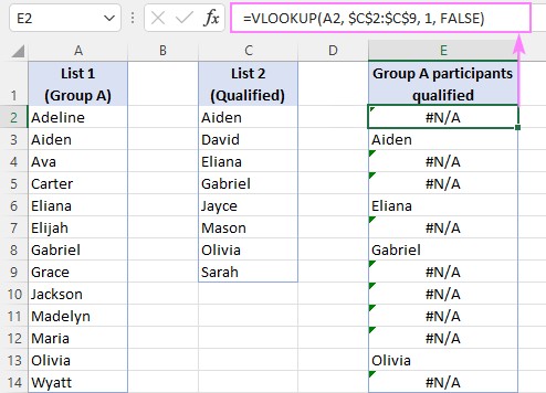
Let’s illustrate with a practical example. Suppose you have two lists: one in column A listing participants and another in column C with qualified participants. You want to know which participants from column A are also in column C.

Enter this formula in cell E2 (assuming your data starts from row 2) and drag it down:

=VLOOKUP(A2, $C$2:$C$9, 1, FALSE)

In this formula:

A2 is the first participant’s name from List 1 (column A).
$C$2:$C$9 is the range of names in List 2 (column C). The dollar signs ($) create absolute references, so the range stays fixed when you drag the formula down.
1 indicates we are interested in a value from the first column of our table_array (which is column C itself in this case, but VLOOKUP needs this argument).
FALSE ensures we are looking for an exact name match.

The formula in column E will display the names of participants from column A that are found in column C. If a name from column A is not in column C, VLOOKUP will return a #N/A error.

Handling #N/A Errors for Cleaner Output

The #N/A errors, while informative for technical users, can be visually distracting or confusing for others. To replace these errors with more user-friendly outputs, we can combine VLOOKUP with error-handling functions like IFNA or IFERROR.

Replacing Errors with Blank Cells

To show a blank cell instead of #N/A when a value isn’t found, use the IFNA function (available in Excel 2013 and later) or IFERROR (available in earlier versions as well, but handles all errors, not just #N/A).

Using IFNA:

=IFNA(VLOOKUP(A2, $C$2:$C$9, 1, FALSE), "")

Using IFERROR:

=IFERROR(VLOOKUP(A2, $C$2:$C$9, 1, FALSE), "")

Both formulas will return a blank cell ("") if VLOOKUP results in a #N/A error, indicating that the value from column A is not found in column C.

Replacing Errors with Custom Text

For even clearer communication, you can replace #N/A errors with custom text like “Not Found” or “Missing”. For example:

=IFNA(VLOOKUP(A2, $C$2:$C$9, 1, FALSE), "Not Qualified")

This will display “Not Qualified” in column E for participants from column A who are not in the qualified list (column C).

Comparing Columns Across Different Excel Sheets

Often, the data you need to compare resides in different worksheets within the same Excel workbook. VLOOKUP handles this seamlessly by allowing you to reference ranges in other sheets.

Assume List 1 is in column A of “Sheet1” and List 2 is in column A of “Sheet2”. To compare them and find matches against List 2, use this formula in “Sheet1”:

=IFNA(VLOOKUP(A2, Sheet2!$A$2:$A$9, 1, FALSE), "")

Notice Sheet2!$A$2:$A$9. Sheet2! specifies that the range $A$2:$A$9 is located in “Sheet2”. Excel automatically handles sheet references when you select ranges with your mouse while building the formula.

Extracting Common Values (Matches) from Two Columns

The basic VLOOKUP formula, especially when combined with IFNA or IFERROR, helps identify common values by showing the matches and leaving blanks (or custom text) for mismatches. To get a clean list of only the common values, you can filter out the blanks.

Using Auto-Filter to List Matches

After applying the VLOOKUP formula (e.g., =IFNA(VLOOKUP(A2, $C$2:$C$9, 1, FALSE), "")) in a helper column (like column E in our examples), you can use Excel’s Auto-Filter to display only the rows where column E is not blank.

Select the header of the column with your VLOOKUP formulas (e.g., cell E1).
Go to the “Data” tab in the Excel ribbon and click “Filter”.
Click the dropdown arrow in the header of column E.
Uncheck “(Blanks)” and click “OK”.

This will filter your data to show only the rows where VLOOKUP found a match, effectively giving you a list of common values.

Using the FILTER Function for Dynamic Lists of Matches

For users of Excel for Microsoft 365 and Excel 2021, the FILTER function offers a dynamic way to extract common values without manual filtering.

=FILTER(A2:A14, IFNA(VLOOKUP(A2:A14, C2:C9, 1, FALSE), "")<>"")

This formula directly returns a list of common values. Here’s how it works:

FILTER(A2:A14, ...): This starts the FILTER function, indicating we want to filter List 1 (A2:A14).
IFNA(VLOOKUP(A2:A14, C2:C9, 1, FALSE), "")<>"": This is the criteria for filtering. It uses VLOOKUP to check if each value in A2:A14 exists in C2:C9. IFNA turns #N/A errors into blank strings. <>"" then checks if the result is not a blank string (meaning a match was found).

Alternatively, using ISNA:

=FILTER(A2:A14, ISNA(VLOOKUP(A2:A14, C2:C9, 1, FALSE))=FALSE)

This is similar but uses ISNA to check for #N/A errors directly. =FALSE means we only want to include values where VLOOKUP did not return an error (i.e., found a match).

Another approach with XLOOKUP (Excel 365 and 2021):

=FILTER(A2:A14, XLOOKUP(A2:A14, C2:C9, C2:C9,"")<>"")

XLOOKUP simplifies this further due to its optional if_not_found argument, allowing us to handle missing values internally.

Identifying Missing Values (Differences) Between Two Columns

To find values that are in the first column but not in the second, we need to identify where VLOOKUP returns #N/A errors. We can use ISNA and IF functions for this.

=IF(ISNA(VLOOKUP(A2, $C$2:$C$9, 1, FALSE)), A2, "")

This formula checks if VLOOKUP returns #N/A using ISNA. If ISNA is TRUE (meaning #N/A error, value not found), the IF function returns the value from column A (the missing value). Otherwise, it returns a blank string.

Again, you can use Auto-Filter to remove the blank rows and get a clean list of missing values.

For dynamic lists in Excel 365 and 2021, use FILTER with ISNA:

=FILTER(A2:A14, ISNA(VLOOKUP(A2:A14, C2:C9, 1, FALSE)))

This FILTER formula directly returns a list of values from column A that are not found in column C.

Or with XLOOKUP:

=FILTER(A2:A14, XLOOKUP(A2:A14, C2:C9, C2:C9,"")="")

This uses XLOOKUP to return blank strings for missing values, and FILTER selects values from List 1 where XLOOKUP returned a blank string.

Labeling Matches and Differences

To add labels directly in your worksheet indicating whether each value in the first list is present in the second, combine VLOOKUP with IF and ISNA.

=IF(ISNA(VLOOKUP(A2, $D$2:$D$9, 1, FALSE)), "Not in List 2", "In List 2")

This formula labels each item in column A as “In List 2” if it’s found in column D, and “Not in List 2” otherwise. You can customize the labels as needed.

Similarly, you can use MATCH function for labeling:

=IF(ISNA(MATCH(A2, $D$2:$D$9, 0)), "Not in List 2", "In List 2")

MATCH function finds the position of a value in a range, and ISNA(MATCH(...)) checks if a match is found (no error) or not (error).

VLOOKUP for Comparing Columns and Returning Values from a Third Column

VLOOKUP’s original purpose shines when you need to compare columns and return related data. Imagine you have two tables: one with participant names and another with qualified participants and their scores. You want to find the score of each participant from the first table who is also in the qualified list.

=VLOOKUP(A3, $D$3:$E$10, 2, FALSE)

Here:

A3 is the participant’s name from the first table.
$D$3:$E$10 is the table array from the second table, containing names (column D) and scores (column E, the second column in the array).
2 is the col_index_num, indicating we want to return the value from the second column (scores).

To handle cases where a participant is not in the qualified list and avoid #N/A errors, use IFNA:

=IFNA(VLOOKUP(A3, $D$3:$E$10, 2, FALSE), "Not Available")

This will return the score if the name is found, and “Not Available” otherwise.

Alternatives like INDEX MATCH and XLOOKUP are also excellent for this task:

=IFNA(INDEX($E$3:$E$10, MATCH(A3, $D$3:$D$10, 0)), "Not Available")

=XLOOKUP(A3, $D$3:$D$10, $E$3:$E$10, "Not Available")

For dynamic lists of qualified participants and their scores (Excel 365 and 2021):

=FILTER(A3:B15, B3:B15<>"") (assuming scores are in column B and blanks indicate not qualified in the original data).

Advanced Comparison Tools

For users who frequently perform data comparison in Excel, specialized tools can significantly enhance efficiency. Ablebits Ultimate Suite offers powerful add-ins:

Compare Tables: Quickly identify duplicates and unique values across columns, lists, or tables.
Compare Two Sheets: Highlight differences between two entire worksheets for detailed analysis.
Compare Multiple Sheets: Analyze and highlight differences across multiple sheets simultaneously.

These tools can save considerable time and effort compared to manual formula-based comparisons, especially for large datasets or complex comparisons.

Downloadable Practice Workbook

To practice the techniques discussed in this guide, download our example workbook:

VLOOKUP in Excel to compare columns – examples (.xlsx file)

By mastering VLOOKUP and these column comparison techniques, you’ll significantly improve your Excel data analysis capabilities and work more efficiently with lists and datasets.