VLOOKUP: Your Go-To Excel Formula to Compare Two Columns

Comparing data across two columns is a common task in Excel, whether you’re reconciling lists, identifying discrepancies, or simply trying to find common ground. While there are several ways to approach this, the VLOOKUP function stands out as a versatile and efficient method. This guide will walk you through various scenarios of using VLOOKUP to compare two columns, helping you pinpoint matches, uncover missing data, and ultimately gain deeper insights from your spreadsheets.

Basic VLOOKUP Formula for Column Comparison

At its heart, VLOOKUP is designed to search for a specific value in a column (the “lookup column”) and return a corresponding value from the same row in another column. When comparing two columns, we leverage VLOOKUP to check if values from one column exist in the other.

Here’s the fundamental VLOOKUP formula structure for comparing two columns:

=VLOOKUP(lookup_value, table_array, col_index_num, range_lookup)

Let’s break down each argument in the context of comparing columns:

lookup_value: This is the value you want to search for. When comparing columns, this will be the first cell in your first column (List 1) that you want to check against the second column.
table_array: This is the second column (List 2), the range where you want to search for the lookup_value. It’s crucial to use absolute references (e.g., $C$2:$C$9) for this argument so that the range remains fixed when you copy the formula down.
col_index_num: This argument specifies which column to return a value from within the table_array. Since we are simply checking for the existence of the lookup_value in the table_array (List 2, which is a single column in this case), we use 1.
range_lookup: This determines whether to find an approximate or exact match. For comparing columns to find exact matches (which is usually the case), we use FALSE (or 0).

Example: Identifying Qualified Participants

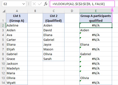
Imagine you have two lists: Column A (List 1) contains the names of all participants, and Column C (List 2) lists participants who qualified for the next round. You want to determine which participants from List 1 qualified.

In cell E2 (or any empty column next to List 1), enter the formula:

=VLOOKUP(A2, $C$2:$C$9, 1, FALSE)
Drag the fill handle (the small square at the bottom-right of cell E2) down to apply the formula to all names in List 1.

Interpreting the Results

If a name from List 1 is found in List 2, the VLOOKUP formula will return that name in column E. This signifies a match – the participant qualified.
If a name from List 1 is not found in List 2, VLOOKUP will return a #N/A error. This indicates a mismatch – the participant did not qualify.

While the basic formula works, the #N/A errors might seem untidy. Let’s explore how to handle them.

Cleaning Up #N/A Errors: Displaying Blanks or Custom Text

The #N/A error is Excel’s way of saying “Value Not Available.” While technically correct, it might not be the most user-friendly output. We can use the IFNA or IFERROR functions to replace these errors with more meaningful displays, such as blank cells or custom text.

Using IFNA to Display Blank Cells

The IFNA function specifically handles #N/A errors. It takes two arguments: the value to check for an error and the value to return if an error is found.

To replace #N/A errors with blank cells, wrap the VLOOKUP formula within IFNA:

=IFNA(VLOOKUP(A2, $C$2:$C$9, 1, FALSE), "")

This formula now returns:

The matched name if found in List 2.
A blank cell (“”) if the name is not found (resulting in a #N/A error from VLOOKUP).

Using IFNA to Display Custom Text

You can also replace errors with custom text to provide more context. For example, to display “Not in List 2” for missing values:

=IFNA(VLOOKUP(A2, $C$2:$C$9, 1, FALSE), "Not in List 2")

Now, instead of #N/A or blanks, you’ll see “Not in List 2” for participants who did not qualify.

Comparing Columns Across Different Excel Sheets

Often, the columns you need to compare reside on different sheets within the same Excel workbook. VLOOKUP handles this seamlessly using external references.

Example: Lists on Sheet1 and Sheet2

Assume List 1 is in column A of “Sheet1” and List 2 is in column A of “Sheet2”. To compare them and find matches, you would use the following formula in Sheet1, starting in cell B2 (or any empty column):

=IFNA(VLOOKUP(A2, Sheet2!$A$2:$A$9, 1, FALSE), "")

Key takeaway: Sheet2!$A$2:$A$9 is the external reference, specifying the range on “Sheet2”. Excel automatically creates these references when you select ranges from other sheets while building your formula.

Extracting Common Values (Matches)

The formulas so far identify matches and differences. But what if you only want a clean list of the common values – the entries present in both columns?

Using Filter to Isolate Matches

One straightforward approach is to use Excel’s Filter feature.

Apply the basic VLOOKUP (or IFNA-enhanced VLOOKUP) formula as described earlier to identify matches and differences, resulting in a column with matched values and #N/A errors (or blanks/custom text).
Select the header of the column containing your VLOOKUP formulas.
Go to the Data tab on the Excel ribbon and click Filter.
Click the filter dropdown arrow in the VLOOKUP results column.
Uncheck the “(Blanks)” or “(#N/A)” option (depending on whether you used IFNA or the basic VLOOKUP). Click OK.

This will filter the list to display only the rows where VLOOKUP found a match, effectively giving you a list of common values.

Dynamic Arrays (Excel 365 and 2021): Using FILTER Function

For users of Excel 365 and Excel 2021, the FILTER function provides a dynamic and formula-based way to extract common values.

=FILTER(A2:A14, IFNA(VLOOKUP(A2:A14, C2:C9, 1, FALSE), "")<>"")

Explanation:

FILTER(A2:A14, ...): This instructs Excel to filter the range A2:A14 (List 1).
IFNA(VLOOKUP(A2:A14, C2:C9, 1, FALSE), "")<>"": This is the criteria for the filter.
- VLOOKUP(A2:A14, C2:C9, 1, FALSE): This VLOOKUP now operates on the entire range A2:A14 at once (thanks to dynamic arrays). It returns an array of matches and #N/A errors.
- IFNA(..., ""): Replaces #N/A errors with blank strings.
- ...<>"": Checks if the result is not a blank string. This condition is TRUE for matches and FALSE for mismatches.

The FILTER function then returns only the values from A2:A14 where the criteria is TRUE – the common values.

Alternative with ISNA and FILTER

Another approach using FILTER and ISNA:

=FILTER(A2:A14, ISNA(VLOOKUP(A2:A14, C2:C9, 1, FALSE))=FALSE)

Here, ISNA(VLOOKUP(...)) returns TRUE if VLOOKUP results in #N/A (mismatch) and FALSE if it finds a match. We filter for FALSE to keep only the matches.

Using XLOOKUP for Simpler Formulas (Excel 365 and 2021)

XLOOKUP, the modern successor to VLOOKUP, simplifies this further:

=FILTER(A2:A14, XLOOKUP(A2:A14, C2:C9, C2:C9,"")<>"")

XLOOKUP has a built-in if_not_found argument. We use "" (blank string) to handle missing values directly within XLOOKUP, making the formula cleaner.

Finding Missing Values (Differences)

To find values present in List 1 but missing from List 2, we need to identify the #N/A errors (or blanks if using IFNA) and extract the corresponding values from List 1.

Using IF and ISNA

Core VLOOKUP: Start with the basic VLOOKUP: VLOOKUP(A2, $C$2:$C$9, 1, FALSE)
ISNA Check: Wrap it in ISNA: ISNA(VLOOKUP(A2, $C$2:$C$9, 1, FALSE)) This returns TRUE for #N/A errors (missing values) and FALSE for matches.
IF Function: Use IF to return the value from List 1 if ISNA is TRUE (missing value) and a blank string if FALSE (match):

=IF(ISNA(VLOOKUP(A2, $C$2:$C$9, 1, FALSE)), A2, "")

This formula will return:
- The value from List 1 if it’s not found in List 2 (a missing value).
- A blank cell if the value is found in List 2 (a match).

Dynamic Arrays (Excel 365 and 2021): FILTER for Missing Values

For dynamic lists of missing values:

=FILTER(A2:A14, ISNA(VLOOKUP(A2:A14, C2:C9, 1, FALSE)))

This FILTER formula uses the ISNA(VLOOKUP(...)) part directly as the include argument. It filters A2:A14 to include only rows where ISNA(VLOOKUP(...)) is TRUE – the missing values.

XLOOKUP Alternative for Missing Values

Using XLOOKUP with FILTER for missing values:

=FILTER(A2:A14, XLOOKUP(A2:A14, C2:C9, C2:C9,"")="")

Here, we filter for values in List 1 where XLOOKUP returns a blank string (meaning not found).

Labeling Matches and Differences

Sometimes, you need to explicitly label each item in List 1 as either “Match” (present in List 2) or “Difference” (not in List 2).

IF and ISNA with VLOOKUP for Labels

=IF(ISNA(VLOOKUP(A2, $D$2:$D$9, 1, FALSE)), "Not in List 2", "In List 2")

This formula uses ISNA(VLOOKUP(...)) to check for mismatches. If a mismatch (TRUE), it returns “Not in List 2”; otherwise (FALSE, a match), it returns “In List 2”. You can customize the labels as needed (e.g., “Qualified”/”Not Qualified”).

MATCH Function for Labeling

The MATCH function can also identify matches and differences:

=IF(ISNA(MATCH(A2, $D$2:$D$9, 0)), "Not in List 2", "In List 2")

MATCH(A2, $D$2:$D$9, 0) attempts to find A2 within $D$2:$D$9. It returns the position of the match if found, and #N/A if not found. ISNA(MATCH(...)) then works similarly to ISNA(VLOOKUP(...)) for labeling.

Returning Values from a Third Column Based on Comparison

VLOOKUP’s primary strength is not just comparing columns but also retrieving related information. Imagine you have two tables: one with participant names and another with qualified participants and their scores. You want to compare names and, for qualified participants, retrieve their scores.

Standard VLOOKUP for Retrieving Related Data

=VLOOKUP(A3, $D$3:$E$10, 2, FALSE)

Here:

A3 is the participant name from the first table.
$D$3:$E$10 is the second table, containing names (column D) and scores (column E – the 2nd column in the table array).
2 is the col_index_num, telling VLOOKUP to return the value from the second column of the table_array (the scores).

Handling Errors and Returning Custom “Not Available” Text

=IFNA(VLOOKUP(A3, $D$3:$E$10, 2, FALSE), "Not available")

This formula uses IFNA to display “Not available” for participants not found in the second table, instead of #N/A errors.

INDEX/MATCH and XLOOKUP Alternatives

=IFNA(INDEX($E$3:$E$10, MATCH(A3, $D$3:$D$10, 0)), "") (INDEX/MATCH)

=XLOOKUP(A3, $D$3:$D$10, $E$3:$E$10, "") (XLOOKUP)

These formulas offer alternative, and often more flexible, ways to achieve the same result. INDEX/MATCH is powerful when dealing with more complex lookups, and XLOOKUP is a modern and often simpler option, especially for Excel 365 and 2021 users.

Filtering Results with Scores

=FILTER(A3:B15, B3:B15<>"")

This FILTER formula (assuming scores are in column B) can be used to display only the participants from the first table who have scores (i.e., those who qualified), effectively filtering out blanks in the score column.

Conclusion

VLOOKUP is a robust tool for comparing two columns in Excel, offering a wide range of functionalities from simple match/mismatch detection to extracting related data and creating dynamic lists. By mastering the techniques outlined in this guide, you can efficiently analyze and compare your data, gaining valuable insights and streamlining your spreadsheet tasks. Whether you’re identifying common entries, pinpointing differences, or retrieving associated information, VLOOKUP empowers you to effectively compare columns and unlock the power of your Excel data.