When to Use Balanced Accuracy for Multiclass Classification: A Comprehensive Guide

In the realm of machine learning, evaluating model performance is as crucial as building the model itself. Metrics act as our compass, guiding us to understand how effectively our models are learning patterns from data. Before deployment, ensuring a model achieves satisfactory performance is paramount, requiring iterative refinement to strike the ideal balance between underfitting and overfitting.

While a plethora of metrics exist for gauging machine learning model performance, this article will focus on balanced accuracy, particularly its significance in the context of multiclass classification. You might sometimes hear the term “normalized accuracy,” and while conceptually related, “balanced accuracy” is the more widely accepted and precise term in the field. We’ll delve into why balanced accuracy is a vital metric, especially when dealing with the complexities of multiclass problems and imbalanced datasets.

Understanding the Landscape: Types of Machine Learning Problems

Machine learning problems broadly fall into two categories: Classification and Regression. Classification deals with predicting discrete categories or labels, while Regression focuses on predicting continuous numerical values.

Classification further branches into:

Binary Classification: Predicting one of two possible classes. Often, one class represents a “normal” state, and the other an “abnormal” state. A classic example is fraud detection, where transactions are classified as either fraudulent or legitimate. In such cases, the “abnormal” class (fraudulent transactions) is often underrepresented, making robust evaluation metrics even more critical.
Multiclass Classification: Predicting among three or more classes. Multiclass problems can sometimes be tackled by extending binary classifiers using strategies like One-vs-Rest or One-vs-One, effectively breaking down the problem into multiple binary classification tasks.

The Role of Evaluation Metrics

Imagine building a sophisticated machine learning model only to realize after deployment that its performance is far from expectations. This scenario underscores the critical need for model evaluation. A common pitfall for beginners is neglecting to rigorously evaluate their models after development, leading to potentially unreliable and inefficient deployments.

An evaluation metric serves as a quantitative measure of a model’s performance after training. It provides feedback on how well the model generalizes to unseen data. The iterative process of model building involves training, evaluating using metrics, and refining the model based on the metric feedback until the desired level of accuracy is achieved.

Choosing the appropriate evaluation metric is paramount. Relying on a single metric might not always paint a complete picture, and a combination of metrics often offers a more nuanced understanding of model performance. The choice of metric is inherently tied to the nature of the problem – classification, regression, etc. – and should align with the specific goals and requirements of the modeling task. In this discussion, we will concentrate on metrics relevant to classification problems.

It’s important to distinguish between evaluation metrics and loss functions. Loss functions guide the model during training, quantifying the error the model makes and helping it adjust its parameters. Metrics, on the other hand, are used to assess the model’s effectiveness after training is complete.

One invaluable tool for understanding model performance, although not a metric itself, is the Confusion Matrix.

Demystifying the Confusion Matrix

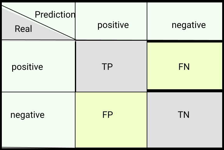
The confusion matrix is a table that visualizes the performance of a classification model. For an N-class classification problem, it’s an N x N matrix that summarizes the counts of correct and incorrect predictions for each class. It reveals not only how well the model is performing overall but also where it excels and where it falters, highlighting areas for potential improvement and the types of errors the model tends to make.

Alt Text: Structure of a confusion matrix for binary classification with True Positives (TP), True Negatives (TN), False Positives (FP), and False Negatives (FN) clearly labeled.

In a binary classification context, the confusion matrix components are:

TP (True Positive): The model correctly predicts the positive class.
TN (True Negative): The model correctly predicts the negative class.
FP (False Positive): The model incorrectly predicts the positive class (Type I error).
FN (False Negative): The model incorrectly predicts the negative class (Type II error).

Let’s now explore some common classification metrics, starting with the most basic: accuracy.

Common Classification Metrics: Accuracy, Recall, Precision, F1-Score, and ROC AUC

Accuracy

Accuracy, often referred to as standard accuracy, is perhaps the most intuitive classification metric. It represents the proportion of correctly classified instances out of the total number of instances.

Accuracy = (TP + TN) / (TP + FN + FP + TN)

Accuracy is calculated directly from the counts in the confusion matrix, focusing on the overall correctness of predictions without considering the predicted probabilities themselves.

Recall (Sensitivity)

Recall, also known as sensitivity or True Positive Rate (TPR), quantifies the model’s ability to identify all actual positive instances. It measures the proportion of correctly predicted positives out of all actual positives.

Recall = TP / (TP + FN)

In multiclass classification, recall can be calculated for each class individually. Macro recall is often used, which is the average recall across all classes.

Macro Recall = (Recall_{Class 1} + Recall_{Class 2} + … + Recall_{Class n}) / n

In binary classification, recall is synonymous with sensitivity, highlighting the model’s sensitivity to positive instances.

Precision

Precision measures the proportion of correctly predicted positive instances out of all instances predicted as positive. It answers the question: “Of all the instances the model labeled as positive, how many were actually positive?”

Precision = TP / (TP + FP)

Precision focuses on the accuracy of positive predictions, penalizing false positives.

F1-Score

The F1-score is the harmonic mean of precision and recall, providing a balanced measure that considers both false positives and false negatives. It’s particularly useful when dealing with imbalanced datasets where simply maximizing precision or recall might be misleading.

F1 = 2 (Precision Recall) / (Precision + Recall)

The F1-score strives for a balance between precision and recall, making it a robust metric when class distributions are uneven.

ROC AUC (Receiver Operating Characteristic Area Under the Curve)

ROC AUC summarizes the trade-off between the True Positive Rate (sensitivity) and the False Positive Rate (FPR) across various classification thresholds. A higher ROC AUC indicates better model performance in distinguishing between classes. ROC AUC is particularly valuable when the class balance is relatively even.

Unlike the previous metrics, ROC AUC is not directly derived from the confusion matrix counts alone. It considers the predicted probabilities or scores assigned to instances, requiring the ROC curve to be plotted, which visualizes the TPR against FPR at different thresholds.

Balanced Accuracy: Addressing Imbalanced Datasets in Multiclass Classification

Balanced accuracy is a metric designed to provide a more realistic performance assessment, especially when dealing with imbalanced datasets in both binary and multiclass classification. It addresses the limitations of standard accuracy, which can be inflated by a model’s ability to correctly classify the majority class in imbalanced scenarios.

The Formula for Balanced Accuracy

Balanced Accuracy = (Sensitivity + Specificity) / 2

Sensitivity: As previously defined, also known as Recall or True Positive Rate (TPR).

Sensitivity = TP / (TP + FN)

Specificity: Also known as the True Negative Rate (TNR), measures the proportion of correctly identified negative instances out of all actual negatives.

Specificity = TN / (TN + FP)

To calculate balanced accuracy in Python, you can use the balanced_accuracy_score function from the sklearn.metrics module:

from sklearn.metrics import balanced_accuracy_score
bal_acc = balanced_accuracy_score(y_test, y_pred)

Balanced Accuracy in Binary Classification: A Fraud Detection Example

Consider a fraud detection scenario where fraudulent transactions are rare compared to legitimate ones. This is a classic example of an imbalanced dataset. In such cases, standard accuracy can be misleadingly high.

Let’s imagine a binary classifier with the following confusion matrix:

Let’s calculate standard accuracy:

Accuracy = (TP + TN) / (TP + FN + FP + TN) = (20 + 5000) / (20 + 70 + 30 + 5000) ≈ 98.05%

An accuracy of 98.05% might seem impressive at first glance. However, in an imbalanced dataset, high accuracy can be deceptive. The model might be achieving this high score simply by predominantly predicting the majority class (legitimate transactions) and largely ignoring the minority class (fraudulent transactions). It might not be effectively identifying fraudulent activities at all.

Now, let’s calculate balanced accuracy for the same classifier:

Sensitivity = TP / (TP + FN) = 20 / (20 + 70) ≈ 22.2%

Specificity = TN / (TN + FP) = 5000 / (5000 + 30) ≈ 99.4%

Balanced Accuracy = (Sensitivity + Specificity) / 2 = (22.2 + 99.4) / 2 ≈ 60.80%

The balanced accuracy of 60.80% paints a far less optimistic picture than the 98.05% standard accuracy. Balanced accuracy reveals that while the model is excellent at identifying legitimate transactions (high specificity), it is very poor at detecting fraudulent ones (low sensitivity). By giving equal weight to both classes, balanced accuracy provides a more realistic assessment of performance in imbalanced scenarios.

Balanced Accuracy for Multiclass Classification: Extending the Concept

Just as in binary classification, balanced accuracy is highly valuable in multiclass classification, especially when dealing with class imbalance. In the multiclass setting, balanced accuracy is defined as the average of the recall scores for each class, which is equivalent to the macro-average of recall. For balanced datasets, balanced accuracy and standard accuracy tend to converge.

Let’s consider a multiclass classification problem with four classes (P, Q, R, S) and an imbalanced class distribution, represented by the confusion matrix below:

The corresponding True Positives (TP), False Positives (FP), True Negatives (TN), and False Negatives (FN) derived from this matrix are summarized as:

Calculating standard accuracy:

Accuracy = (TP + TN) / (TP + FP + FN + TN)

TP = 10 + 545 + 11 + 3 = 569

FP = 175 + 104 + 39 + 50 = 368

TN = 695 + 248 + 626 + 874 = 2443

FN = 57 + 40 + 261 + 10 = 368

Accuracy = (569 + 2443) / (569 + 368 + 368 + 2443) ≈ 0.803 or 80.3%

Again, an accuracy of 80.3% might seem reasonable. However, closer inspection of the confusion matrix reveals that classes P and S are significantly imbalanced, and the model appears to perform poorly on these classes.

Let’s compute balanced accuracy:

Balanced Accuracy = (Recall_P + Recall_Q + Recall_R + Recall_S) / 4

Recall for each class is calculated as:

Recall = TP / (TP + FN)

Recall_P = 10 / (10 + 57) ≈ 0.054 (Very low recall for class P)
Recall_Q = 545 / (545 + 40) ≈ 0.932
Recall_R = 11 / (11 + 261) ≈ 0.040 (Very low recall for class R)
Recall_S = 3 / (3 + 10) ≈ 0.231 (Low recall for class S)

Balanced Accuracy = (0.054 + 0.932 + 0.040 + 0.231) / 4 ≈ 0.3143 or 31.43%

The balanced accuracy of 31.43% is significantly lower than the standard accuracy of 80.3%. This stark difference highlights the issue: the model, while achieving high overall accuracy due to good performance on the majority class Q, is actually performing poorly on the minority classes P, R, and S. Balanced accuracy effectively reveals this weakness by giving equal weight to the recall of each class. This insight is crucial for guiding further model improvement, suggesting the need for more data or specific techniques to improve performance on classes P, S, and R.

Balanced Accuracy vs. Classification Accuracy: Choosing the Right Metric

Standard accuracy is a suitable metric when the dataset is reasonably balanced and when all classes are equally important. However, in imbalanced datasets, it can be misleading and provide an inflated view of performance. This can lead to the accuracy paradox, where high accuracy doesn’t necessarily translate to a useful model.

Consider this confusion matrix for an imbalanced binary classification problem:

Calculating standard accuracy:

Accuracy = (TP + TN) / (TP + FN + FP + TN) = (0 + 190) / (0 + 10 + 0 + 190) = 190 / 200 = 0.95 or 95%

Accuracy is 95%, seemingly excellent. However, let’s examine balanced accuracy:

Sensitivity = TP / (TP + FN) = 0 / (0 + 10) = 0%

Specificity = TN / (TN + FP) = 190 / (190 + 0) = 100%

Balanced Accuracy = (Sensitivity + Specificity) / 2 = (0 + 1) / 2 = 0.5 or 50%

Balanced accuracy is 50%, indicating performance no better than random guessing. This reveals the critical flaw: the model is only predicting the negative class and completely failing to identify any positive instances, despite the high standard accuracy. In such scenarios, balanced accuracy is a far more informative metric.

Balanced accuracy is essential when dealing with imbalanced datasets, as it provides a more realistic measure of performance across all classes, regardless of their frequency. If the dataset is well-balanced, standard accuracy and balanced accuracy will tend to converge to similar values.

Balanced Accuracy vs. F1-Score: Complementary Metrics

Both balanced accuracy and the F1-score are often used for imbalanced classification, but they emphasize different aspects of performance.

F1-Score prioritizes the balance between precision and recall, focusing on the positive class.

F1 = 2 (Precision Recall) / (Precision + Recall)

Balanced Accuracy balances sensitivity and specificity, giving equal importance to both positive and negative classes in binary classification, or macro-averaging recall across all classes in multiclass.

Balanced Accuracy = (Specificity + Recall) / 2

F1-score does not explicitly consider true negatives (TN) in its calculation. In situations where accurately identifying negative instances is also crucial, balanced accuracy becomes more relevant.
When both positive and negative classes are equally important, balanced accuracy is often a more reliable metric than F1-score.
F1-score is a good choice when the primary focus is on achieving high precision and recall for the positive class, even at the expense of potentially lower performance on the negative class.

Consider this scenario: a dataset with 1000 negative samples and 10 positive samples. A model predicts 15 positive samples (5 true positives, 10 false positives) and 985 negative samples (990 true negatives, 5 false negatives).

Calculating F1-score and balanced accuracy:

Precision = 5 / 15 ≈ 0.33

Sensitivity (Recall) = 5 / 10 = 0.5

Specificity = 990 / 1000 = 0.99

F1-score = 2 (0.5 0.33) / (0.5 + 0.33) ≈ 0.4

Balanced Accuracy = (0.5 + 0.99) / 2 ≈ 0.745

In this case, balanced accuracy (0.745) is higher than the F1-score (0.4), reflecting that balanced accuracy gives more weight to the correctly classified negatives.

Now consider another scenario where there are no true negatives:

Precision = 5 / 15 ≈ 0.33

Sensitivity (Recall) = 5 / 10 = 0.5

Specificity = 0 / 10 = 0

F1-score = 2 (0.5 0.33) / (0.5 + 0.33) ≈ 0.4

Balanced Accuracy = (0.5 + 0) / 2 = 0.25

Notice that the F1-score remains unchanged (approximately 0.4), while balanced accuracy drops significantly from 0.745 to 0.25. This demonstrates that F1-score is less sensitive to changes in true negatives, whereas balanced accuracy is more responsive to performance across both positive and negative classes.

Balanced Accuracy vs. ROC AUC: Different Perspectives

ROC AUC and balanced accuracy both provide valuable insights, but they differ in their approach and suitability depending on the specific problem.

Balanced accuracy is calculated on discrete predicted classes, while ROC AUC is calculated on predicted probability scores for the positive class. ROC AUC requires probability outputs and cannot be directly computed from confusion matrix counts alone.
For highly imbalanced datasets, balanced accuracy is often preferred over ROC AUC. ROC AUC can be less sensitive to class imbalance, especially when imbalance is severe. Small changes in correct/incorrect predictions can lead to significant score variations in ROC AUC in highly skewed datasets.
If you need a range of probability estimates for observations, ROC AUC is more appropriate as it averages performance across all possible classification thresholds. However, if the goal is to output discrete class labels, and class imbalance is a concern, balanced accuracy is often a better choice.
ROC AUC evaluates the model’s ability to distinguish between classes across all possible thresholds, making it suitable when you care about the model’s overall ranking ability and trade-offs between sensitivity and specificity. Balanced accuracy focuses on the average recall per class (multiclass) or balance between sensitivity and specificity (binary) at a specific threshold (often the default threshold of 0.5 for binary classification).

Implementing Balanced Accuracy with Multiclass Classification: Practical Example

To illustrate the practical application of balanced accuracy and other metrics in a multiclass classification setting, let’s consider an example using the Diamonds dataset from Seaborn. The task is to predict the ‘cut’ quality of diamonds, a multiclass classification problem.

(The original article provides a code example using Python, scikit-learn, and Neptune. For brevity, I will summarize the key steps and concepts here. Refer to the original article for the full code implementation.)

Environment Setup: Install necessary libraries (pandas, scikit-learn, seaborn, Neptune for experiment tracking).
Data Loading: Load the Diamonds dataset using Seaborn.
Data Exploration and Cleaning: Analyze class distribution of the ‘cut’ variable (target). Observe class imbalance (e.g., ‘Ideal’ cut being the majority class). Handle categorical features using one-hot encoding and label encoding as appropriate.
Data Splitting: Split data into training and testing sets, using stratified sampling to maintain class proportions in both sets.
Model Training: Train a Random Forest Classifier for multiclass classification.
Prediction and Evaluation:
- Generate predictions on the test set.
- Calculate various metrics: standard accuracy, balanced accuracy, recall, precision, F1-score, ROC AUC (using one-vs-rest approach for multiclass).
- Use Neptune or a similar experiment tracking tool to log and visualize these metrics for different model configurations (e.g., varying number of estimators in Random Forest).
- Plot ROC curves and confusion matrices for visual analysis of performance.

(Refer to the original article’s code for detailed implementation of these steps, including Neptune experiment tracking.)

The practical example demonstrates how to calculate and track balanced accuracy alongside other metrics in a multiclass classification scenario. By monitoring balanced accuracy, especially in the context of the imbalanced Diamonds dataset, you can gain a more accurate understanding of model performance compared to relying solely on standard accuracy. Experiment tracking tools like Neptune further enhance this process by providing a centralized platform to visualize and compare metrics across different experiments.

Key Takeaways: When Standard Accuracy Suffices

While balanced accuracy is crucial for imbalanced datasets, standard accuracy remains perfectly valid in certain situations:

Balanced Data: When the class distribution in the dataset is relatively balanced.
Probability-Based Models: When the model’s output is not just a class label but a probability distribution over classes, and the focus is on the overall probabilistic prediction accuracy rather than performance on specific classes.
Preference for Positives: When the primary goal is to maximize performance on the positive class, even if it comes at the expense of performance on the negative class (and the dataset is not severely imbalanced).
Multiclass with Uniform Importance: In multiclass classification problems where all classes are considered equally important, and class imbalance is not a significant concern.

However, when class imbalance is present, or when performance across all classes is equally important, balanced accuracy becomes a more reliable and informative metric.

Summary: Choosing the Right Evaluation Metric

Selecting the appropriate evaluation metrics is a fundamental aspect of machine learning model development. It ensures that you are not only building a model but also effectively addressing the problem you set out to solve. Choosing the right metric determines whether your model truly meets the desired performance criteria.

Balanced accuracy is a powerful tool, particularly for imbalanced datasets and multiclass classification, providing a more realistic assessment of model performance than standard accuracy in such scenarios. However, like any metric, it has its strengths and limitations. Understanding these nuances empowers you to make informed decisions about when to prioritize balanced accuracy and when other metrics might be more suitable. By carefully considering the characteristics of your data and the goals of your machine learning task, you can choose the metrics that best guide you toward building robust and effective models.

Thank you for reading!

Product Resource: How Cradle Achieved Experiment Tracking and Data Security Goals With Self-Hosted Neptune
Product Resource: How Veo Eliminated Work Loss With Neptune
Related Article: LLM Evaluation For Text Summarization
Related Article: Building LLM Applications With Vector Databases

Explore more content topics: Computer Vision General LLMOps ML Model Development ML Tools MLOps Natural Language Processing Paper Reflections Product Updates Reinforcement Learning Tabular Data Time Series