How to Use VLOOKUP to Compare Two Lists in Excel

Quickly and accurately identify discrepancies between two datasets using Excel’s VLOOKUP function.

VLOOKUP is a powerful Excel function that allows you to compare two lists and identify matching or missing items. This tutorial provides a step-by-step guide on How To Use Vlookup To Compare Two Lists, enhance your data analysis capabilities, and save valuable time. This method works for Excel 2010, 2013, 2016, 2019, and Excel for Microsoft 365.

Understanding the Basics of Comparing Lists with VLOOKUP

Let’s say you have two spreadsheets: one with your company’s invoice records and another received from a client. Manually comparing these lists to find discrepancies would be time-consuming and prone to errors. VLOOKUP automates this process. It works by looking up a specific value from one list (the lookup value) in another list (the table array). If a match is found, VLOOKUP returns a corresponding value from a specified column in the table array.

For VLOOKUP to work effectively, ensure:

Common Identifier: Both lists must have at least one column with matching data, such as an invoice number, product ID, or employee name. This will serve as your lookup value.
Unique Lookup Value: The lookup value should ideally be unique within the table array to avoid incorrect matches. Invoice numbers are often a good choice due to their uniqueness.
Lookup Value in First Column: VLOOKUP searches for the lookup value in the first column of the table array. Ensure your data is structured accordingly.

Step-by-Step Guide: Using VLOOKUP to Compare Two Lists

1. Naming the Range (Table Array)

First, name the range of data in the list you’ll be searching within. This simplifies the VLOOKUP formula and makes it easier to manage.

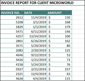
Select the entire data range in the second list (e.g., the client’s invoice report).
In the Name Box (located above the spreadsheet), enter a descriptive name (e.g., “ClientInvoices”) and press Enter.

2. Constructing the VLOOKUP Formula

Now, let’s build the VLOOKUP formula in the first list (e.g., your company’s invoice report).

In the first cell where you want to display the comparison results, enter the following formula:
```
=VLOOKUP(A2,ClientInvoices,1,FALSE) 
```
- A2: The cell containing the lookup value in the first list (e.g., the first invoice number).
- ClientInvoices: The named range of the second list.
- 1: The column number in the named range from which you want to retrieve a value (since we’re just checking for existence, 1 is sufficient).
- FALSE: Specifies an exact match.

3. Handling Errors with ISNA and IF

The initial VLOOKUP formula will return the lookup value if found and an #N/A error if not. Let’s make the results more user-friendly.

Modify the formula to include error handling:
```
=IF(ISNA(VLOOKUP(A2,ClientInvoices,1,FALSE)),"Missing", "")
```
This formula now displays “Missing” if the invoice number is not found in the client’s list and leaves the cell blank if it is found.

4. Highlighting Missing Records with Conditional Formatting

For enhanced visual clarity, use conditional formatting to highlight the missing records.

Select the cells containing the comparison results.
Go to Home > Conditional Formatting > New Rule.
Select Use a formula to determine which cells to format.
Enter the following formula: =ISNA(VLOOKUP(A2,ClientInvoices,1,FALSE))
Choose a formatting style (e.g., fill color) to highlight the cells where the formula evaluates to TRUE (meaning the record is missing).

Conclusion

By leveraging VLOOKUP’s capabilities and incorporating error handling and conditional formatting, you can efficiently compare two lists in Excel, identify discrepancies, and streamline your data analysis workflow. This technique is invaluable for tasks like data reconciliation, invoice matching, and inventory management.