How to Use VLOOKUP to Compare Two Columns in Excel: A Comprehensive Guide

Comparing two columns of data in Excel is a common task for data analysis, list management, and report generation. Whether you need to identify matching entries, find unique values, or pinpoint discrepancies between datasets, Excel offers several powerful tools. Among these, the VLOOKUP function stands out as a versatile method for column comparison. This guide will explore how to effectively use VLOOKUP to compare two columns in Excel, enabling you to find both commonalities and differences in your data.

Understanding Basic VLOOKUP for Column Comparison

VLOOKUP is primarily known for retrieving data from a table based on a lookup value. However, its ability to search for a value in a column and return a corresponding value (or an error if not found) makes it perfectly suited for comparing two columns. The fundamental idea is to use VLOOKUP to search for each value from the first column in the second column.

Here’s the basic syntax of the VLOOKUP function:

=VLOOKUP(lookup_value, table_array, col_index_num, [range_lookup])

To use VLOOKUP for comparing two columns, you’ll apply it as follows:

lookup_value: This will be the first value from your first column (List 1) that you want to search for in the second column (List 2).
table_array: This is the range encompassing your second column (List 2). It’s the area where VLOOKUP will search for the lookup_value.
col_index_num: Since we are only concerned with whether the value exists in the second column or not, and our table_array is just one column, we use 1.
range_lookup: Crucially, set this to FALSE (or 0) to ensure an exact match. We want to know if the exact value from List 1 is present in List 2.

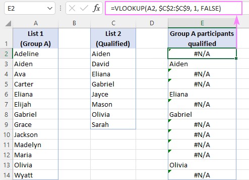
Let’s illustrate with an example. Suppose you have a list of employee IDs in column A (List 1) and a list of IDs of employees who completed training in column C (List 2). You want to determine which employees from List 1 have completed the training. You can use the following formula in cell E2, assuming your List 1 starts from A2 and List 2 is in C2:C9:

=VLOOKUP(A2, $C$2:$C$9, 1, FALSE)

Drag this formula down column E, alongside your List 1.

In the result column (E), if VLOOKUP finds a match (i.e., the employee ID from column A is also in column C), it will return the matched value (the employee ID). If the ID from column A is not found in column C, VLOOKUP will return a #N/A error. This #N/A error is your indicator that the value from List 1 is missing in List 2.

Handling #N/A Errors for Cleaner Results

While #N/A errors effectively highlight differences, they might look unprofessional or confusing in reports. To replace these errors with more user-friendly outputs, you can wrap your VLOOKUP formula within error-handling functions like IFNA or IFERROR.

Using IFNA to Replace #N/A Errors

The IFNA function is specifically designed to handle #N/A errors. If the VLOOKUP formula results in #N/A, IFNA can replace it with a value you specify, such as a blank cell (“”) or custom text.

Here’s how to use IFNA with VLOOKUP to display blank cells instead of #N/A errors:

=IFNA(VLOOKUP(A2, $C$2:$C$9, 1, FALSE), "")

This formula will return the matching value if found, and a blank cell if not found, making your comparison results cleaner and easier to interpret.

You can also replace the blank string "" with custom text to indicate the status more explicitly, for example:

=IFNA(VLOOKUP(A2, $C$2:$C$9, 1, FALSE), "Not in Training List")

This will display “Not in Training List” for employees from List 1 who are not in the training list (List 2).

Comparing Columns Across Different Excel Sheets

Often, the columns you need to compare might reside in different worksheets within the same workbook or even in different workbooks. VLOOKUP can easily handle this by using external references.

To compare columns in different sheets, simply include the sheet name followed by an exclamation mark (!) before the range in the table_array argument.

For example, if List 1 is in column A of “Sheet1” and List 2 is in column A of “Sheet2”, the formula in Sheet1 to compare against Sheet2 would be:

=IFNA(VLOOKUP(A2, Sheet2!$A$2:$A$9, 1, FALSE), "")

Excel automatically handles the sheet references when you select ranges with your mouse while building the formula, making it straightforward to compare data across sheets.

Extracting Common Values (Matches) from Two Columns

The basic VLOOKUP approach shows matches and identifies differences with #N/A errors or blank cells. To specifically extract a list of common values (items present in both columns) without gaps, you can use filtering techniques.

Using AutoFilter to List Common Values

After applying the VLOOKUP formula (with or without error handling) as described earlier, you can use Excel’s AutoFilter to display only the rows where a match is found (i.e., values that are not #N/A or blank if you used IFNA).

Select the header of the column containing your VLOOKUP formulas.
Go to the “Data” tab in the Excel ribbon and click “Filter”.
Click the filter dropdown in your VLOOKUP results column.
Deselect “(Blanks)” if you used IFNA to return blanks, or deselect “(Errors)” if you want to filter out #N/A errors directly. Only rows with matches will remain visible.

Using the FILTER Function for Dynamic Lists of Common Values (Excel 365 and 2021)

For users with Excel 365 or Excel 2021, the FILTER function provides a dynamic way to extract common values. Combined with VLOOKUP, it automatically creates a list of matches that updates as your data changes.

Here’s the formula using FILTER and VLOOKUP to get a dynamic list of common values:

=FILTER(A2:A14, IFNA(VLOOKUP(A2:A14, C2:C9, 1, FALSE), "")<>"")

This formula works by:

VLOOKUP(A2:A14, C2:C9, 1, FALSE): This part attempts to find each value from List 1 (A2:A14) in List 2 (C2:C9). It returns matches or #N/A errors.
IFNA(..., ""): Replaces #N/A errors with blank strings.
...<>"": This checks if the result of IFNA(VLOOKUP(...)) is not a blank string, meaning a match was found. This serves as the criteria for the FILTER function.
FILTER(A2:A14, ...): The FILTER function then returns only the values from List 1 (A2:A14) for which the criteria (a match was found) is true.

Identifying Missing Values (Differences) Between Two Columns

To find values that are in the first column but not in the second (i.e., missing values or differences), you can adapt the VLOOKUP approach.

Using IF and ISNA to Highlight Missing Values

Combine VLOOKUP with the ISNA function and IF function to specifically identify and list the values from List 1 that are not found in List 2.

The formula structure is as follows:

=IF(ISNA(VLOOKUP(A2, $C$2:$C$9, 1, FALSE)), A2, "")

Here’s how it works:

VLOOKUP(A2, $C$2:$C$9, 1, FALSE): As before, this searches for the value from A2 in C2:C9.
ISNA(...): The ISNA function checks if the result of VLOOKUP is #N/A. It returns TRUE if it is #N/A (meaning the value is missing) and FALSE otherwise.
IF(ISNA(...), A2, ""): The IF function uses the result of ISNA. If TRUE (value is missing), it returns the original value from A2 (the missing value). If FALSE (value is found), it returns a blank string.

Using FILTER for Dynamic List of Missing Values (Excel 365 and 2021)

Similar to extracting common values, you can use the FILTER function to dynamically list missing values.

=FILTER(A2:A14, ISNA(VLOOKUP(A2:A14, C2:C9, 1, FALSE)))

This formula directly uses the ISNA(VLOOKUP(...)) result as the include criteria for the FILTER function. It returns only the values from List 1 for which ISNA(VLOOKUP(...)) is TRUE, effectively listing the missing values.

Identifying Matches and Differences with Text Labels

For clearer reporting, you might want to label each item in List 1 as either “Match” (present in List 2) or “Difference” (not present in List 2). You can achieve this by combining VLOOKUP with IF and ISNA.

=IF(ISNA(VLOOKUP(A2, $D$2:$D$9, 1, FALSE)), "Not in List 2", "In List 2")

This formula assigns text labels based on whether VLOOKUP finds a match or returns #N/A. You can customize the labels “Not in List 2” and “In List 2” to be more descriptive for your specific context, such as “Not Qualified” and “Qualified”.

Alternatively, the MATCH function can also be used in a similar way to achieve the same outcome:

=IF(ISNA(MATCH(A2, $D$2:$D$9, 0)), "Not in List 2", "In List 2")

Returning Data from a Third Column Based on Comparison

A primary strength of VLOOKUP is its ability to return related data. When comparing two columns, you can extend VLOOKUP to return a value from a third column associated with the matched value in List 2.

For instance, if you have employee names in column A (List 1) and a table in columns D and E (List 2 and related data) where column D contains names and column E contains department names, you can compare column A names against column D names and return the department from column E for matching names.

=VLOOKUP(A3, $D$3:$E$10, 2, FALSE)

Here, col_index_num is set to 2 because the department names are in the second column of the table_array ($D$3:$E$10). If a name from column A is found in column D, the formula returns the corresponding department from column E. To handle #N/A errors, you can again use IFNA:

=IFNA(VLOOKUP(A3, $D$3:$E$10, 2, FALSE), "Not Available")

This enhanced VLOOKUP application not only compares columns but also leverages the comparison to retrieve and display related information, making it a powerful tool for data analysis and reporting.

Conclusion: VLOOKUP for Efficient Column Comparison in Excel

VLOOKUP is a robust and versatile function for comparing two columns in Excel. Whether you need to find common values, identify differences, or return related data, VLOOKUP provides a range of solutions. By mastering the techniques outlined in this guide, you can efficiently analyze and manage your data, gaining valuable insights from column comparisons. From basic matching to dynamic lists and data retrieval, VLOOKUP is an essential tool in your Excel toolkit for data comparison tasks.

For users seeking even more advanced and streamlined comparison capabilities, Excel add-ins like Ablebits Ultimate Suite offer dedicated tools such as “Compare Tables” and “Compare Two Sheets,” which can further enhance your data comparison workflows.

Practice Workbook for Download:

VLOOKUP in Excel to compare columns – examples (.xlsx file)