How To Do VLOOKUP To Compare Two Columns In Excel

VLOOKUP to compare two columns is a powerful technique for data analysis. At COMPARE.EDU.VN, we provide comprehensive guides to help you master this essential Excel skill. Discover how to efficiently identify matches and differences in your datasets, leading to better data-driven decisions. Improve your spreadsheet skills with VLOOKUP comparisons, data matching, and missing value identification, unlocking the full potential of your data analysis.

1. Understanding the Basics of VLOOKUP for Column Comparison

VLOOKUP, or Vertical Lookup, is a fundamental Excel function that allows you to search for a specific value in the first column of a table and return a corresponding value from another column in the same row. When it comes to comparing two columns, VLOOKUP can be used to check if values in one column exist in another, effectively highlighting matches and differences. This section will cover the basic syntax of VLOOKUP, how it works, and its relevance to comparing columns in Excel.

1.1 VLOOKUP Syntax Explained

The VLOOKUP function has four arguments:

lookup_value: The value you want to search for. This is typically a cell reference in the first column you are comparing.
table_array: The range of cells in which to search for the lookup value. The first column of this range is where the lookup value is searched.
col_index_num: The column number within the table_array from which the matching value will be returned.
range_lookup: A logical value (TRUE or FALSE) that specifies whether you want an approximate or exact match. Use FALSE for an exact match, which is crucial when comparing columns.

Understanding these arguments is crucial for effectively using VLOOKUP to compare columns and extract meaningful insights.
VLOOKUP Syntax in Excel

1.2 How VLOOKUP Works in Column Comparisons

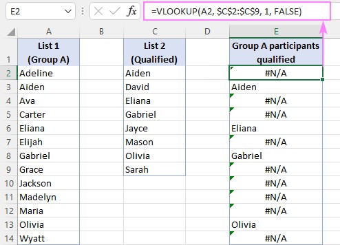
When using VLOOKUP to compare two columns, the function searches for each value from the first column (List 1) in the second column (List 2). If a match is found, VLOOKUP returns the corresponding value from List 2. If no match is found, VLOOKUP returns a #N/A error. This behavior allows you to quickly identify which values from List 1 are present in List 2, and which are missing.

1.3 Why VLOOKUP is Useful for Data Comparison

VLOOKUP is a valuable tool for data comparison because it automates the process of checking for matches and differences between two lists. This is particularly useful when dealing with large datasets where manual comparison would be time-consuming and prone to errors. By using VLOOKUP, you can efficiently identify common values, missing data points, and inconsistencies between two columns, leading to more informed decisions.

2. Step-by-Step Guide: Using VLOOKUP to Compare Two Columns

This section provides a detailed, step-by-step guide on how to use the VLOOKUP function to compare two columns in Excel. We’ll cover how to set up your data, write the VLOOKUP formula, interpret the results, and handle common issues.

2.1 Preparing Your Data

Before you can use VLOOKUP, you need to organize your data properly. Start by ensuring that the two columns you want to compare are in the same Excel sheet or in different sheets within the same workbook. Make sure the data is clean, with no leading or trailing spaces, and that the formatting is consistent.

Open Excel: Launch Microsoft Excel and open the worksheet containing the two columns you want to compare.
Arrange Columns: Ensure that the columns are adjacent to each other or in a layout that makes it easy to reference them in the VLOOKUP formula.
Data Consistency: Check for inconsistencies in the data, such as different capitalization or extra spaces. Use Excel’s TRIM function to remove extra spaces: =TRIM(A1).

2.2 Writing the VLOOKUP Formula

Once your data is prepared, you can write the VLOOKUP formula. Follow these steps:

Select a Cell: Choose an empty column next to your first list. In the first cell of this column, you will enter the VLOOKUP formula.
Enter the Formula: Type the VLOOKUP formula in the selected cell. For example, if you want to compare column A (List 1) with column C (List 2), starting from row 2, the formula would be:
=VLOOKUP(A2, $C$2:$C$100, 1, FALSE)
- A2 is the first value in List 1 that you want to search for in List 2.
- $C$2:$C$100 is the range containing List 2. The dollar signs ($) make the reference absolute, so it doesn’t change when you copy the formula.
- 1 indicates that you want to return the value from the first column of the table_array (List 2).
- FALSE ensures an exact match.
Copy the Formula: Drag the fill handle (the small square at the bottom right of the cell) down to apply the formula to all the cells in List 1.

2.3 Interpreting VLOOKUP Results

After applying the VLOOKUP formula, you will see one of two results in the new column:

Value from List 2: If VLOOKUP finds a match, it will return the corresponding value from List 2. This indicates that the value from List 1 is also present in List 2.
#N/A Error: If VLOOKUP does not find a match, it will return a #N/A error. This indicates that the value from List 1 is not present in List 2.

2.4 Handling Common VLOOKUP Issues

When using VLOOKUP, you may encounter some common issues:

#N/A Errors: These errors occur when VLOOKUP cannot find a match. To handle these errors, you can use the IFNA or IFERROR function to replace the error with a more user-friendly message or a blank cell.
=IFNA(VLOOKUP(A2, $C$2:$C$100, 1, FALSE), "Not Found")
Incorrect Results: Ensure that the range_lookup argument is set to FALSE for exact matches. Also, double-check that your table_array range is correct and includes the entire second list.
Performance Issues: For very large datasets, VLOOKUP can be slow. Consider using other methods, such as Power Query or array formulas, for better performance.

3. Advanced VLOOKUP Techniques for Column Comparison

While the basic VLOOKUP formula is useful for simple comparisons, there are several advanced techniques that can enhance your analysis. This section will explore how to use VLOOKUP with functions like IF, ISNA, and FILTER to perform more complex comparisons.

3.1 Using VLOOKUP with IF and ISNA Functions

Combining VLOOKUP with the IF and ISNA functions allows you to create more informative and customized results. The ISNA function checks whether a value is #N/A, and the IF function allows you to return different values based on a condition.

Identifying Matches and Differences:
Use the following formula to display “Match” if a value from List 1 is found in List 2, and “Difference” if it is not:
=IF(ISNA(VLOOKUP(A2, $C$2:$C$100, 1, FALSE)), "Difference", "Match")
This formula first uses VLOOKUP to search for the value in A2 in the range C2:C100. If VLOOKUP returns #N/A, ISNA returns TRUE, and the IF function displays “Difference”. Otherwise, ISNA returns FALSE, and the IF function displays “Match”.
Returning Custom Text:
You can also return custom text based on whether a match is found. For example, to display “Present in List 2” or “Not in List 2”:
=IF(ISNA(VLOOKUP(A2, $C$2:$C$100, 1, FALSE)), "Not in List 2", "Present in List 2")

3.2 Using VLOOKUP with the FILTER Function

In newer versions of Excel (Microsoft 365 and Excel 2021), the FILTER function can be used with VLOOKUP to dynamically extract matches or differences.

Extracting Common Values:
To get a list of common values between two columns, use the following formula:
=FILTER(A2:A100, NOT(ISNA(VLOOKUP(A2:A100, C2:C100, 1, FALSE))))
This formula uses VLOOKUP to check which values from A2:A100 are present in C2:C100. The ISNA function identifies the #N/A errors (i.e., the values not found), and NOT(ISNA(...)) inverts the result so that FILTER includes only the values that are found.
Extracting Missing Values:
To get a list of values from List 1 that are not present in List 2, use the following formula:
=FILTER(A2:A100, ISNA(VLOOKUP(A2:A100, C2:C100, 1, FALSE)))
This formula uses VLOOKUP to check which values from A2:A100 are present in C2:C100. The ISNA function identifies the #N/A errors, and FILTER includes only those values.

3.3 Comparing Multiple Columns with VLOOKUP

While VLOOKUP is designed to compare two columns at a time, you can extend its functionality to compare multiple columns by nesting multiple VLOOKUP formulas or using helper columns.

Nesting VLOOKUP Formulas:
To check if a value from List 1 is present in either List 2 or List 3, you can nest two VLOOKUP formulas within an OR function inside an IF function:
=IF(OR(NOT(ISNA(VLOOKUP(A2, $C$2:$C$100, 1, FALSE))), NOT(ISNA(VLOOKUP(A2, $D$2:$D$100, 1, FALSE)))), "Present in List 2 or 3", "Not Found")
This formula checks if A2 is present in C2:C100 or D2:D100. If it is found in either list, it returns “Present in List 2 or 3”; otherwise, it returns “Not Found”.
Using Helper Columns:
Another approach is to use helper columns to create a combined list and then use VLOOKUP to compare. For example, you can concatenate List 2 and List 3 into a single helper column and then use VLOOKUP to check against this combined list.

4. Practical Examples of VLOOKUP for Column Comparison

To further illustrate the versatility of VLOOKUP, this section provides practical examples of how it can be used in various scenarios.

4.1 Comparing Customer Lists

Imagine you have two customer lists: one from your CRM system and another from a recent marketing campaign. You want to identify which customers from the marketing campaign are already in your CRM system and which are new.

Data Setup:
- Column A: Customer IDs from the marketing campaign list.
- Column B: Customer IDs from the CRM system list.
VLOOKUP Formula:
In column C, enter the following formula:
=IF(ISNA(VLOOKUP(A2, $B$2:$B$100, 1, FALSE)), "New Customer", "Existing Customer")
This formula checks if the customer ID from the marketing campaign list (Column A) is present in the CRM system list (Column B). If the customer ID is found, it returns “Existing Customer”; otherwise, it returns “New Customer”.

4.2 Comparing Product Catalogs

Suppose you have two product catalogs: one from your main supplier and another from a secondary supplier. You want to identify which products are offered by both suppliers and which are unique to each.

Data Setup:
- Column A: Product SKUs from the main supplier catalog.
- Column B: Product SKUs from the secondary supplier catalog.
VLOOKUP Formula:
In column C, enter the following formula:
=IF(ISNA(VLOOKUP(A2, $B$2:$B$100, 1, FALSE)), "Main Supplier Only", "Offered by Both")
This formula checks if the product SKU from the main supplier catalog (Column A) is present in the secondary supplier catalog (Column B). If the product SKU is found, it returns “Offered by Both”; otherwise, it returns “Main Supplier Only”.

4.3 Comparing Inventory Lists

Consider you have two inventory lists: one from your warehouse management system and another from a recent physical inventory count. You want to identify discrepancies between the two lists.

Data Setup:
- Column A: Item IDs from the warehouse management system list.
- Column B: Item IDs from the physical inventory count list.
VLOOKUP Formula:
In column C, enter the following formula:
=IF(ISNA(VLOOKUP(A2, $B$2:$B$100, 1, FALSE)), "Discrepancy", "Match")
This formula checks if the item ID from the warehouse management system list (Column A) is present in the physical inventory count list (Column B). If the item ID is found, it returns “Match”; otherwise, it returns “Discrepancy”, indicating a potential issue.

5. Alternatives to VLOOKUP for Column Comparison

While VLOOKUP is a powerful tool, it has limitations. This section will explore alternative methods for comparing columns in Excel, including INDEX MATCH, XLOOKUP, and Power Query.

5.1 INDEX MATCH

The INDEX MATCH combination is a flexible alternative to VLOOKUP. It overcomes VLOOKUP’s limitation of only searching in the first column and can return values from columns to the left.

How it Works:
- MATCH finds the position of a value in a range.
- INDEX returns the value at a specific position in a range.
Formula for Comparing Columns:
=IF(ISNA(INDEX($B$2:$B$100, MATCH(A2, $B$2:$B$100, 0))), "Not Found", "Match")
In this formula, MATCH(A2, $B$2:$B$100, 0) finds the position of A2 in B2:B100. If A2 is not found, MATCH returns #N/A, and ISNA returns TRUE. The INDEX function is used to return the results of the match function.

5.2 XLOOKUP

XLOOKUP is a modern replacement for VLOOKUP, available in Excel 365 and Excel 2021. It offers several advantages over VLOOKUP, including the ability to search in any column and return values from any other column without needing to specify a column index number.

Benefits of XLOOKUP:
- More flexible and easier to use than VLOOKUP.
- Can handle errors more gracefully.
- Can search both vertically and horizontally.
Formula for Comparing Columns:
=IF(ISNA(XLOOKUP(A2, $B$2:$B$100, $B$2:$B$100, "Not Found")), "Not Found", "Match")
In this formula, XLOOKUP(A2, $B$2:$B$100, $B$2:$B$100, "Not Found") searches for A2 in B2:B100 and returns the corresponding value from B2:B100. If A2 is not found, it returns “Not Found”.

5.3 Power Query

Power Query is a powerful data transformation and analysis tool built into Excel. It allows you to import data from various sources, clean and transform it, and perform complex comparisons.

Steps to Compare Columns Using Power Query:
- Import Data: Import both lists into Power Query by selecting the data and clicking “Data” > “From Table/Range.”
- Merge Queries: Go to “Home” > “Merge Queries.” Select the two queries (lists) you want to compare.
- Choose Columns: Select the columns to match on (e.g., Customer ID, Product SKU).
- Select Join Kind: Choose the appropriate join kind, such as “Left Outer” to keep all rows from the first list and matching rows from the second list.
- Expand Columns: Expand the columns from the second list that you want to include in the result.
Benefits of Power Query:
- Handles large datasets efficiently.
- Provides a wide range of data transformation options.
- Automates the comparison process with repeatable steps.

6. Optimizing VLOOKUP for Performance and Accuracy

To ensure VLOOKUP performs efficiently and accurately, it’s essential to optimize your formulas and data. This section provides tips on improving VLOOKUP performance and accuracy.

6.1 Using Absolute References

When copying a VLOOKUP formula down a column, it’s crucial to use absolute references for the table_array argument. This prevents the range from shifting as you copy the formula.

How to Use Absolute References:
Use the dollar sign ($) to lock the row and column references. For example, $B$2:$B$100 ensures that the range B2:B100 remains constant when the formula is copied.

6.2 Sorting Data

VLOOKUP can perform faster when the lookup column in the table_array is sorted in ascending order, especially when using approximate matches (range_lookup = TRUE). However, for accurate comparisons, it’s best to use exact matches (range_lookup = FALSE), which don’t require sorted data.

6.3 Minimizing Volatile Functions

Volatile functions, such as NOW() and RAND(), recalculate every time the worksheet changes, which can slow down VLOOKUP performance. Avoid using volatile functions in your VLOOKUP formulas if possible.

6.4 Handling Large Datasets

For very large datasets, VLOOKUP can become slow. Consider the following strategies:

Use INDEX MATCH or XLOOKUP: These functions can be faster than VLOOKUP in certain scenarios.
Use Power Query: Power Query is designed to handle large datasets efficiently.
Optimize Data Types: Ensure that the data types in the lookup column are consistent. For example, if you are comparing numbers, make sure they are all formatted as numbers and not text.
Reduce Worksheet Calculation: Set the calculation mode to manual (Formulas > Calculation Options > Manual) and recalculate only when necessary.

7. Common Mistakes to Avoid When Using VLOOKUP

To ensure accurate and efficient VLOOKUP usage, it’s essential to avoid common mistakes. This section highlights these mistakes and provides solutions.

7.1 Incorrect Range References

One of the most common mistakes is using incorrect range references for the table_array argument. Always double-check that the range includes the entire lookup table and that the column references are correct.

7.2 Forgetting Absolute References

When copying a VLOOKUP formula, forgetting to use absolute references for the table_array can cause the range to shift, leading to incorrect results. Always use dollar signs ($) to lock the row and column references.

7.3 Using Approximate Match with Unsorted Data

Using approximate match (range_lookup = TRUE) with unsorted data can lead to unpredictable results. If you want to use approximate match, make sure the lookup column in the table_array is sorted in ascending order. However, for accurate comparisons, it’s best to use exact matches (range_lookup = FALSE).

7.4 Data Type Mismatches

Data type mismatches between the lookup_value and the lookup column in the table_array can cause VLOOKUP to fail. For example, if the lookup_value is a number and the lookup column contains text, VLOOKUP may not find a match. Ensure that the data types are consistent.

7.5 Not Handling Errors

Not handling errors, such as #N/A, can make your worksheet look unprofessional and confuse users. Use the IFNA or IFERROR function to replace errors with more user-friendly messages or blank cells.

8. Real-World Applications of VLOOKUP in Various Industries

VLOOKUP is a versatile tool with applications across various industries. This section explores real-world examples of how VLOOKUP can be used in different sectors.

8.1 Finance

In finance, VLOOKUP can be used to:

Compare financial statements: Compare data from different periods to identify trends and discrepancies.
Analyze stock prices: Retrieve historical stock prices and compare them to current prices.
Manage customer accounts: Match customer IDs from different systems to consolidate account information.

8.2 Marketing

In marketing, VLOOKUP can be used to:

Analyze campaign performance: Compare data from different marketing channels to identify the most effective strategies.
Segment customer lists: Match customer data from different sources to create targeted marketing lists.
Track lead generation: Compare lead lists from different sources to identify duplicate leads.

8.3 Human Resources

In human resources, VLOOKUP can be used to:

Manage employee data: Match employee IDs from different systems to consolidate personnel information.
Track training records: Compare employee training records to identify employees who need additional training.
Analyze performance reviews: Compare performance review data from different periods to identify trends and areas for improvement.

8.4 Supply Chain Management

In supply chain management, VLOOKUP can be used to:

Compare inventory lists: Match inventory data from different systems to identify discrepancies.
Track order fulfillment: Compare order data from different sources to ensure timely fulfillment.
Analyze supplier performance: Compare supplier data from different periods to identify the most reliable suppliers.

9. Tips and Tricks for Mastering VLOOKUP

To become a VLOOKUP master, it’s essential to practice and learn advanced techniques. This section provides tips and tricks for mastering VLOOKUP.

9.1 Practice Regularly

The best way to master VLOOKUP is to practice regularly. Work through different examples and scenarios to build your skills and confidence.

9.2 Learn Advanced Techniques

Explore advanced VLOOKUP techniques, such as using VLOOKUP with IF, ISNA, and FILTER functions. These techniques allow you to perform more complex comparisons and customize your results.

9.3 Understand Error Handling

Master error handling by using the IFNA or IFERROR function to replace errors with more user-friendly messages or blank cells. This makes your worksheets look more professional and easier to understand.

9.4 Explore Alternatives

Explore alternatives to VLOOKUP, such as INDEX MATCH, XLOOKUP, and Power Query. These tools can be more efficient and flexible in certain scenarios.

9.5 Stay Updated

Stay updated with the latest Excel features and functions. Microsoft regularly releases new updates that can improve your VLOOKUP skills and efficiency.

10. Conclusion: Enhancing Data Analysis with VLOOKUP

VLOOKUP is a powerful and versatile tool for comparing columns in Excel. By mastering VLOOKUP and its advanced techniques, you can efficiently identify matches and differences in your data, leading to better insights and more informed decisions. Whether you’re in finance, marketing, human resources, or supply chain management, VLOOKUP can help you streamline your data analysis and improve your overall productivity. Remember to practice regularly, explore advanced techniques, and stay updated with the latest Excel features to become a VLOOKUP master.

Are you ready to take your data analysis skills to the next level? Visit COMPARE.EDU.VN today to discover more comprehensive guides and resources. Whether you’re comparing product catalogs, customer lists, or inventory data, COMPARE.EDU.VN provides the tools and knowledge you need to make informed decisions. Don’t let data discrepancies hold you back. Start your journey to data mastery with COMPARE.EDU.VN today.

For more information, contact us at:
Address: 333 Comparison Plaza, Choice City, CA 90210, United States
Whatsapp: +1 (626) 555-9090
Website: compare.edu.vn

FAQ: Frequently Asked Questions about VLOOKUP

1. What is VLOOKUP used for?

VLOOKUP is used to search for a specific value in the first column of a table and return a corresponding value from another column in the same row. It is commonly used to compare data, retrieve information, and automate tasks in Excel.

2. How do I use VLOOKUP to compare two columns?

To compare two columns using VLOOKUP, use the VLOOKUP function to search for values from the first column in the second column. If a match is found, VLOOKUP returns the corresponding value from the second column. If no match is found, VLOOKUP returns a #N/A error.

3. What does #N/A mean in VLOOKUP?

The #N/A error in VLOOKUP means that the function could not find a match for the lookup_value in the table_array. This can be due to various reasons, such as incorrect range references, data type mismatches, or the value not being present in the lookup table.

4. How do I fix #N/A errors in VLOOKUP?

To fix #N/A errors in VLOOKUP, use the IFNA or IFERROR function to replace the error with a more user-friendly message or a blank cell. For example:
=IFNA(VLOOKUP(A2, $B$2:$B$100, 1, FALSE), "Not Found")

5. What is the difference between VLOOKUP and HLOOKUP?

VLOOKUP (Vertical Lookup) searches for a value in the first column of a table and returns a corresponding value from another column in the same row. HLOOKUP (Horizontal Lookup) searches for a value in the first row of a table and returns a corresponding value from another row in the same column.

6. Can VLOOKUP search to the left?

No, VLOOKUP can only search in the first column of the table_array and return values from columns to the right. To search to the left, use the INDEX MATCH combination or XLOOKUP.

7. What is the alternative to VLOOKUP?

Alternatives to VLOOKUP include INDEX MATCH, XLOOKUP, and Power Query. These tools can be more flexible and efficient in certain scenarios.

8. How do I use VLOOKUP with multiple criteria?

VLOOKUP is designed to work with a single criterion. To use VLOOKUP with multiple criteria, you can create a helper column that concatenates the criteria and then use VLOOKUP to search for the concatenated value.

9. What is the difference between exact match and approximate match in VLOOKUP?

Exact match (range_lookup = FALSE) requires an exact match between the lookup_value and the values in the lookup column. Approximate match (range_lookup = TRUE) finds the closest match in the lookup column. For accurate comparisons, it’s best to use exact matches.

10. How do I speed up VLOOKUP in Excel?

To speed up VLOOKUP in Excel, use absolute references, sort the data in the lookup column (if using approximate match), minimize volatile functions, optimize data types, and consider using INDEX MATCH, XLOOKUP, or Power Query for large datasets.