Comparing data across two spreadsheets can be a daunting task. This is especially true when dealing with large datasets. Learn How To Do A Vlookup To Compare Two Sheets and reconcile data differences using COMPARE.EDU.VN. By understanding this powerful function, you can quickly identify matching, non-matching, and missing data, streamlining your workflow and ensuring data accuracy.
1. Understanding the Need for Sheet Comparison
In various professional and academic settings, the need to compare two spreadsheets arises frequently. Whether it’s reconciling financial data, comparing sales reports, or verifying customer information, the ability to efficiently compare two sets of data is crucial. This is where a VLOOKUP formula shines. It allows you to quickly cross-reference data between two sheets based on a common identifier.
The process of comparing data is often challenging due to:
- Volume of Data: Large datasets make manual comparison time-consuming and prone to error.
- Data Inconsistencies: Variations in data entry, formatting, or updates can lead to discrepancies.
- Time Constraints: Meeting deadlines often requires quick and accurate data comparison.
Organizations and individuals must utilize efficient methods to overcome these challenges. VLOOKUP offers a robust solution by automating the comparison process, reducing errors, and saving valuable time.
2. What is VLOOKUP and Why Use It?
VLOOKUP (Vertical Lookup) is an Excel function that searches for a value in the first column of a range and returns a value from a specified column in the same row. It’s a powerful tool for comparing data across two sheets because it allows you to quickly find matching values based on a unique identifier.
Key advantages of using VLOOKUP include:
- Efficiency: Automates the process of finding and comparing data.
- Accuracy: Reduces the risk of human error in data comparison.
- Versatility: Can be used with various types of data, including text, numbers, and dates.
- Speed: Quickly processes large datasets, providing results in seconds.
VLOOKUP works by taking a lookup value, searching for it in the first column of a table array, and then returning a corresponding value from another column in the same row. This makes it ideal for comparing two sheets where you have a common identifier, such as customer ID, product code, or invoice number.
3. Essential Preparation Steps Before Using VLOOKUP
Before diving into the VLOOKUP formula, proper preparation is crucial to ensure accurate and reliable results. This involves setting up your data in a structured and consistent manner.
3.1. Ensure Data Consistency
One of the most critical steps is ensuring that your data is consistent across both sheets. This includes:
- Data Types: Ensure that the data types in the lookup column (e.g., customer ID) are the same in both sheets. Inconsistencies in data types (e.g., number vs. text) can cause VLOOKUP to fail.
- Formatting: Standardize the formatting of dates, numbers, and text. Different formatting can lead to VLOOKUP not recognizing matching values.
- Case Sensitivity: VLOOKUP is not case-sensitive by default. However, if case sensitivity is important, consider using a helper column with a formula to convert all values to the same case (e.g., UPPER or LOWER).
By ensuring data consistency, you minimize the risk of errors and ensure that VLOOKUP accurately identifies matching values.
3.2. Identify a Unique Identifier
A unique identifier is a column that contains unique values for each row in your data. This is crucial for VLOOKUP because it allows the function to accurately match records between the two sheets. Common examples of unique identifiers include:
- Customer ID: A unique code assigned to each customer.
- Product Code: A unique code assigned to each product.
- Invoice Number: A unique number assigned to each invoice.
- Employee ID: A unique code assigned to each employee.
If your data doesn’t already have a unique identifier, you may need to create one. This can be done by concatenating multiple columns or generating a unique code using a formula.
3.3. Organize Your Sheets
Organizing your sheets in a clear and structured manner will make it easier to work with VLOOKUP. This includes:
- Naming Sheets: Give your sheets descriptive names (e.g., “Sheet1” becomes “SalesData2023”, “Sheet2” becomes “SalesData2024”).
- Headers: Ensure that each column has a clear and descriptive header.
- Data Range: Define the data range that you want to use with VLOOKUP. Avoid including empty rows or columns in your range.
By organizing your sheets, you make it easier to understand your data and use VLOOKUP effectively.
4. Step-by-Step Guide: How to Do a VLOOKUP
With your data prepared, you can now use VLOOKUP to compare your two sheets. Here’s a step-by-step guide:
4.1. Open the First Sheet
Start by opening the first sheet that contains the data you want to compare. This sheet will be the basis for your VLOOKUP formula.
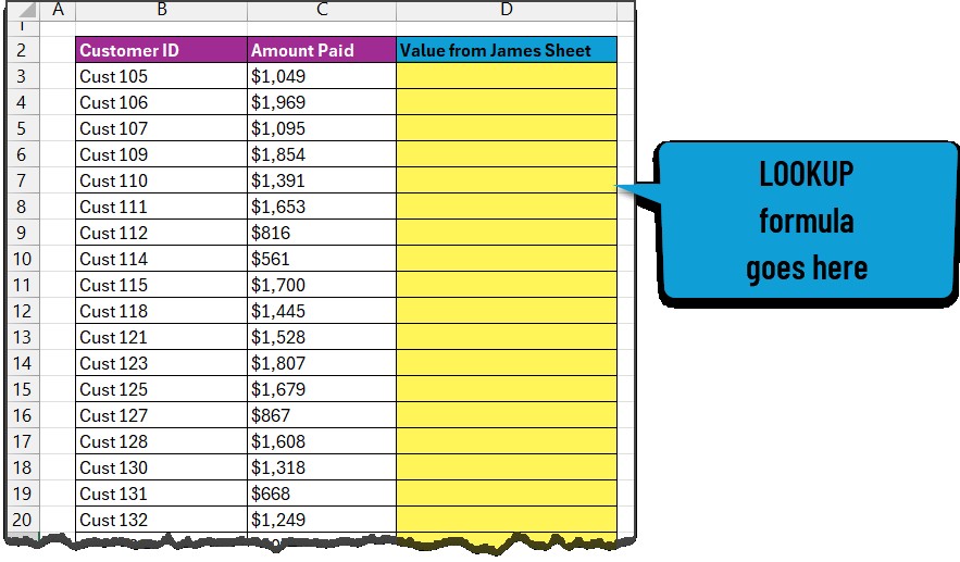
4.2. Select the Cell for the VLOOKUP Formula
Choose an empty column next to the data in your first sheet. Select the first cell in this column where you want to enter the VLOOKUP formula. This cell will display the result of the VLOOKUP function.
4.3. Write the VLOOKUP Formula
Enter the VLOOKUP formula into the selected cell. The basic syntax of the VLOOKUP formula is:
=VLOOKUP(lookup_value, table_array, col_index_num, [range_lookup])Let’s break down each component of the formula:
- lookup_value: The value you want to search for in the first column of the table array. This is typically a cell containing the unique identifier.
- table_array: The range of cells that contains the data you want to search in. This is typically the entire data range of the second sheet.
- col_index_num: The column number in the table array from which you want to return a value. This is the column containing the data you want to compare.
- [range_lookup]: An optional argument that specifies whether you want to find an exact match (FALSE) or an approximate match (TRUE). In most cases, you’ll want to use FALSE to find an exact match.
Here’s an example of a VLOOKUP formula:
=VLOOKUP(A2, 'Sheet2'!A:B, 2, FALSE)In this example:
- A2: The lookup value is in cell A2 of the first sheet.
- ‘Sheet2’!A:B: The table array is the entire range of columns A and B in the second sheet.
- 2: The column index number is 2, meaning you want to return a value from the second column of the table array.
- FALSE: You want to find an exact match.
4.4. Drag the Formula Down
After entering the VLOOKUP formula in the first cell, drag the fill handle (the small square at the bottom-right corner of the cell) down to apply the formula to the remaining rows in your data. This will automatically adjust the lookup value for each row.
5. Interpreting VLOOKUP Results: Handling Errors
After applying the VLOOKUP formula, it’s important to understand how to interpret the results and handle any errors that may occur.
5.1. Understanding Matching Values
When VLOOKUP finds a matching value in the second sheet, it will return the corresponding value from the specified column. This indicates that the data matches between the two sheets for that particular record.
5.2. Dealing with #N/A Errors
The most common error you’ll encounter with VLOOKUP is the #N/A error. This error indicates that VLOOKUP could not find a matching value in the second sheet for the specified lookup value. This can happen for a variety of reasons:
- Missing Data: The lookup value may not exist in the second sheet.
- Data Inconsistencies: The data type or formatting of the lookup value may be different in the two sheets.
- Typographical Errors: There may be a typo in the lookup value.
To handle #N/A errors, you can use the IFERROR function to display a more user-friendly message. The IFERROR function allows you to specify a value to return if a formula results in an error.
Here’s an example of how to use the IFERROR function with VLOOKUP:
=IFERROR(VLOOKUP(A2, 'Sheet2'!A:B, 2, FALSE), "Not Found")In this example, if VLOOKUP returns an #N/A error, the IFERROR function will display the message “Not Found”.
5.3. Using ISNA Function
Alternatively, you can use the ISNA function to identify #N/A errors and perform different actions based on whether an error exists. The ISNA function returns TRUE if a value is an #N/A error and FALSE otherwise.
Here’s an example of how to use the ISNA function with VLOOKUP:
=IF(ISNA(VLOOKUP(A2, 'Sheet2'!A:B, 2, FALSE)), "Not Found", VLOOKUP(A2, 'Sheet2'!A:B, 2, FALSE))In this example, if VLOOKUP returns an #N/A error, the ISNA function will return TRUE, and the IF function will display the message “Not Found”. Otherwise, the IF function will display the result of the VLOOKUP function.
6. Advanced Techniques: Combining VLOOKUP with Other Functions
To enhance the functionality of VLOOKUP, you can combine it with other Excel functions. Here are a few examples:
6.1. Using IF to Compare Values
You can use the IF function to compare the values returned by VLOOKUP with the corresponding values in the first sheet. This allows you to quickly identify records where the data does not match.
Here’s an example of how to use the IF function with VLOOKUP:
=IF(VLOOKUP(A2, 'Sheet2'!A:B, 2, FALSE) = B2, "Match", "No Match")In this example, the IF function compares the value returned by VLOOKUP with the value in cell B2 of the first sheet. If the values match, the IF function displays the message “Match”. Otherwise, it displays the message “No Match”.
6.2. Using Conditional Formatting to Highlight Differences
Conditional formatting allows you to automatically format cells based on certain criteria. You can use conditional formatting to highlight records where the data does not match between the two sheets.
Here’s how to use conditional formatting with VLOOKUP:
- Select the range of cells that you want to format.
- Go to Home > Conditional Formatting > New Rule.
- Select “Use a formula to determine which cells to format”.
- Enter the following formula:
=VLOOKUP($A2, 'Sheet2'!$A:$B, 2, FALSE) <> $B2- Click the Format button and choose the formatting options you want to use to highlight the differences.
- Click OK to apply the conditional formatting.
This will highlight all the records where the data does not match between the two sheets.
6.3. Using MATCH to Find Column Index
Instead of manually entering the column index number in the VLOOKUP formula, you can use the MATCH function to dynamically find the column index based on the column header. This is useful when the column order in the second sheet may change.
Here’s an example of how to use the MATCH function with VLOOKUP:
=VLOOKUP(A2, 'Sheet2'!A:C, MATCH("ColumnHeader", 'Sheet2'!A1:C1, 0), FALSE)In this example, the MATCH function searches for the column header “ColumnHeader” in the range A1:C1 of the second sheet and returns the column index number. This column index number is then used in the VLOOKUP formula.
7. Alternatives to VLOOKUP
While VLOOKUP is a powerful tool for comparing two sheets, there are also other functions and techniques you can use. Here are a few alternatives:
7.1. XLOOKUP
XLOOKUP is a newer function that is available in Excel 365 and later versions. It is similar to VLOOKUP but offers several advantages:
- No Need to Specify Column Index: XLOOKUP automatically returns the corresponding value from the same row in the return array.
- Handles Errors Automatically: XLOOKUP has a built-in error handling feature that allows you to specify a value to return if no match is found.
- Supports Vertical and Horizontal Lookups: XLOOKUP can be used to perform both vertical and horizontal lookups.
Here’s an example of how to use XLOOKUP to compare two sheets:
=XLOOKUP(A2, 'Sheet2'!A:A, 'Sheet2'!B:B, "Not Found")In this example:
- A2: The lookup value is in cell A2 of the first sheet.
- ‘Sheet2’!A:A: The lookup array is the entire column A in the second sheet.
- ‘Sheet2’!B:B: The return array is the entire column B in the second sheet.
- “Not Found”: The value to return if no match is found.
7.2. INDEX and MATCH
The combination of INDEX and MATCH functions provides a more flexible alternative to VLOOKUP. INDEX returns a value from a specified row and column in a range, while MATCH returns the position of a value in a range.
Here’s an example of how to use INDEX and MATCH to compare two sheets:
=INDEX('Sheet2'!B:B, MATCH(A2, 'Sheet2'!A:A, 0))In this example:
- ‘Sheet2’!B:B: The range from which to return a value.
- MATCH(A2, ‘Sheet2’!A:A, 0): The MATCH function searches for the value in cell A2 of the first sheet in the range A:A of the second sheet and returns the position of the match.
- INDEX: The INDEX function returns the value from the specified row (returned by MATCH) in the range B:B of the second sheet.
7.3. Power Query
Power Query is a powerful data transformation and analysis tool that is built into Excel. It allows you to import data from multiple sources, clean and transform the data, and then load it into a single sheet. You can use Power Query to compare two sheets by merging them based on a common identifier.
Here’s a general outline of how to use Power Query to compare two sheets:
- Import Data: Import both sheets into Power Query using Data > Get & Transform Data > From Table/Range.
- Merge Queries: Merge the two queries based on a common identifier using Home > Merge Queries.
- Expand Columns: Expand the columns you want to compare from the second sheet.
- Compare Values: Add a custom column to compare the values from the two sheets using a formula.
- Load Data: Load the transformed data into a new sheet.
8. Best Practices for Effective Sheet Comparison
To ensure accurate and efficient sheet comparison, follow these best practices:
- Regularly Update Data: Keep your data up-to-date to avoid discrepancies.
- Validate Data: Implement data validation rules to ensure data consistency.
- Document Your Formulas: Add comments to your formulas to explain their purpose and functionality.
- Test Your Formulas: Thoroughly test your formulas to ensure they are working correctly.
- Use Consistent Formatting: Use consistent formatting across all your sheets.
- Secure Your Data: Protect your data from unauthorized access.
- Back Up Your Data: Regularly back up your data to prevent data loss.
9. Streamline Data Comparison with COMPARE.EDU.VN
Comparing two sheets using VLOOKUP can be a powerful way to reconcile data. However, complex comparisons or large datasets can still be time-consuming. For a more streamlined and efficient solution, consider using COMPARE.EDU.VN.
COMPARE.EDU.VN offers comprehensive comparison tools that simplify the process of analyzing and reconciling data across multiple sources. Whether you’re comparing financial statements, sales reports, or any other type of data, COMPARE.EDU.VN can help you quickly identify differences, highlight discrepancies, and ensure data accuracy.
Key benefits of using COMPARE.EDU.VN include:
- Advanced Comparison Algorithms: Quickly identify differences and similarities in your data.
- Customizable Comparison Settings: Tailor the comparison process to your specific needs.
- Interactive Reports: Visualize your comparison results with interactive charts and graphs.
- Secure Data Handling: Protect your data with advanced security measures.
- User-Friendly Interface: Easily navigate and use the platform.
10. Real-World Examples of VLOOKUP in Sheet Comparison
To illustrate the practical applications of VLOOKUP in sheet comparison, here are a few real-world examples:
- Reconciling Bank Statements: Compare transactions in your bank statement with transactions in your accounting software.
- Comparing Sales Reports: Compare sales data from different regions or time periods.
- Verifying Customer Information: Compare customer data from different sources to ensure accuracy and completeness.
- Analyzing Inventory Data: Compare inventory levels from different warehouses or storage locations.
- Validating Financial Data: Compare financial data from different departments or subsidiaries.
In each of these examples, VLOOKUP can be used to quickly and accurately identify matching, non-matching, and missing data, helping you to make informed decisions and improve your business processes.
FAQ: Common Questions About VLOOKUP and Sheet Comparison
Q1: Can VLOOKUP compare data in different Excel files?
Yes, VLOOKUP can compare data in different Excel files. You just need to specify the file name in the table_array argument. For example, =VLOOKUP(A2, '[OtherFile.xlsx]Sheet1'!$A:$B, 2, FALSE).
Q2: How do I handle case sensitivity in VLOOKUP?
VLOOKUP is not case-sensitive by default. To handle case sensitivity, you can use a helper column with a formula to convert all values to the same case (e.g., UPPER or LOWER). Then, use the helper column in your VLOOKUP formula.
Q3: Can VLOOKUP return multiple values?
No, VLOOKUP can only return one value. To return multiple values, you can use multiple VLOOKUP formulas or use the INDEX and MATCH functions.
Q4: How do I compare data in multiple columns using VLOOKUP?
To compare data in multiple columns, you can use multiple VLOOKUP formulas, one for each column. Alternatively, you can use Power Query to merge the data and then compare the values.
Q5: What is the difference between VLOOKUP and HLOOKUP?
VLOOKUP searches for a value in the first column of a range, while HLOOKUP searches for a value in the first row of a range.
Q6: How do I improve the performance of VLOOKUP with large datasets?
To improve the performance of VLOOKUP with large datasets, you can sort the data in the table_array by the lookup column. This can significantly speed up the search process.
Q7: Can I use VLOOKUP to compare data in different data types?
Yes, you can use VLOOKUP to compare data in different data types. However, you need to ensure that the data types are compatible. For example, you may need to convert numbers to text or vice versa.
Q8: How do I find the last match in VLOOKUP?
VLOOKUP always returns the first match it finds. To find the last match, you can reverse the order of the data in the table_array and then use VLOOKUP.
Q9: Can I use wildcards in VLOOKUP?
Yes, you can use wildcards in VLOOKUP to find partial matches. The wildcard characters are * (matches any number of characters) and ? (matches a single character).
Q10: How do I troubleshoot errors in VLOOKUP?
To troubleshoot errors in VLOOKUP, check the following:
- Ensure that the lookup value exists in the table_array.
- Ensure that the data types are consistent.
- Ensure that the column index number is correct.
- Check for typos in the formula.
- Use the IFERROR function to handle errors.
Conclusion: Simplify Sheet Comparison with VLOOKUP and COMPARE.EDU.VN
Mastering VLOOKUP is an invaluable skill for anyone working with data in Excel. By following the steps outlined in this guide, you can effectively compare two sheets, identify discrepancies, and ensure data accuracy.
However, for more complex comparisons or when dealing with large datasets, consider leveraging the power of COMPARE.EDU.VN. With its advanced comparison algorithms, customizable settings, and user-friendly interface, COMPARE.EDU.VN simplifies the process of analyzing and reconciling data, saving you time and ensuring accurate results.
Ready to streamline your sheet comparison process and make data-driven decisions with confidence? Visit COMPARE.EDU.VN today to explore our comprehensive comparison tools and discover how we can help you unlock the full potential of your data. For inquiries or support, contact us at 333 Comparison Plaza, Choice City, CA 90210, United States. You can also reach us via Whatsapp at +1 (626) 555-9090. Let compare.edu.vn be your partner in data excellence!