How to Create a Pivot Table to Compare Data

Data analysis is crucial for informed decision-making. How To Create A Pivot Table To Compare Data becomes essential for uncovering insights and patterns. COMPARE.EDU.VN provides comprehensive guides, tools, and resources to help you master data comparison techniques, empowering you to make confident choices. This article explains data summarization and visualization.

1. Understanding Pivot Tables: A Foundation for Data Comparison

A pivot table is a powerful tool in spreadsheet programs like Microsoft Excel and Google Sheets that allows you to summarize and analyze large datasets. It enables you to quickly rearrange and aggregate data to identify trends, patterns, and relationships. Think of it as a dynamic data analysis tool that lets you explore your data from different angles.

1.1. What is a Pivot Table?

A pivot table is an interactive data summarization tool. It extracts, organizes, and summarizes data from a source table or range, allowing you to analyze it in various ways. It provides a flexible way to view your data, making it easier to identify trends and patterns. You can easily change the arrangement of the data to see different perspectives, hence the term “pivot.”

1.2. Key Components of a Pivot Table

Understanding the key components is crucial for effectively using pivot tables. These components define how your data is organized and analyzed.

Rows: These are the categories or fields that you want to display horizontally in your pivot table. They often represent different groups or segments of your data.
Columns: These are the categories or fields that you want to display vertically in your pivot table. They can represent different time periods, product categories, or other dimensions.
Values: These are the numerical data that you want to summarize in your pivot table. They can be sums, averages, counts, or other calculations.
Filters: These allow you to narrow down the data that is displayed in your pivot table. You can filter by specific categories, time periods, or other criteria.

1.3. Benefits of Using Pivot Tables for Data Comparison

Pivot tables offer numerous benefits for data comparison. Here are a few key advantages:

Efficiency: Pivot tables can quickly summarize large datasets, saving you time and effort compared to manual calculations.
Flexibility: You can easily rearrange the data in a pivot table to explore different perspectives and identify hidden patterns.
Clarity: Pivot tables present data in a clear and concise format, making it easier to understand and interpret.
Interactivity: You can interact with a pivot table by filtering, sorting, and drilling down into the data to gain deeper insights.
Customization: Pivot tables can be customized to meet your specific needs, allowing you to focus on the data that is most important to you.

2. Step-by-Step Guide: Creating a Pivot Table in Excel

Creating a pivot table in Excel is a straightforward process. Follow these steps to get started:

2.1. Preparing Your Data

Before creating a pivot table, it is crucial to organize your data properly. Ensure that your data is in a tabular format with clear column headers. This will make it easier for Excel to interpret your data and create an effective pivot table.

Clean Your Data: Remove any errors, inconsistencies, or missing values from your data.
Format Your Data: Ensure that your data is formatted correctly. Dates should be in date format, numbers should be in number format, and text should be in text format.
Use Clear Column Headers: Use clear and descriptive column headers to identify each field in your data.

2.2. Inserting a Pivot Table

Once your data is prepared, you can insert a pivot table.

Select Your Data: Select the entire range of data that you want to include in your pivot table.
Go to the Insert Tab: In the Excel ribbon, click on the “Insert” tab.
Click PivotTable: In the “Tables” group, click on the “PivotTable” button.
Choose Your Data Source: In the “Create PivotTable” dialog box, confirm that the selected range is correct.
Choose Where to Place the Pivot Table: Select whether you want to place the pivot table in a new worksheet or an existing worksheet.
Click OK: Click “OK” to create the pivot table.

2.3. Building Your Pivot Table: Adding Fields

After inserting the pivot table, you can start building it by adding fields to the different areas.

PivotTable Fields Pane: The “PivotTable Fields” pane will appear on the right side of the screen. This pane lists all the column headers from your data source.
Drag Fields to Areas: Drag the fields from the “PivotTable Fields” pane to the different areas of the pivot table: “Rows,” “Columns,” “Values,” and “Filters.”
- Rows: Drag the fields that you want to display as rows in your pivot table.
- Columns: Drag the fields that you want to display as columns in your pivot table.
- Values: Drag the fields that you want to summarize in your pivot table.
- Filters: Drag the fields that you want to use as filters for your pivot table.

2.4. Configuring Value Field Settings

The “Values” area is where you configure how your data is summarized. You can change the calculation method, number format, and other settings.

Right-Click on a Value Field: In the pivot table, right-click on a value field.
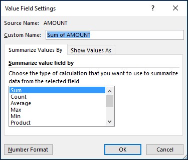
Select Value Field Settings: In the context menu, select “Value Field Settings.”
Choose a Calculation Method: In the “Value Field Settings” dialog box, choose a calculation method from the “Summarize Values By” tab. Options include “Sum,” “Count,” “Average,” “Max,” “Min,” and more.
Change the Number Format: In the “Value Field Settings” dialog box, click on the “Number Format” button to change the number format for the value field.
Click OK: Click “OK” to apply the settings.

2.5. Filtering Your Data

Filtering allows you to focus on specific subsets of your data.

Use the Filter Area: Drag fields to the “Filters” area in the “PivotTable Fields” pane.
Click the Filter Dropdown: In the pivot table, click the dropdown arrow next to the filter field.
Select Filter Criteria: Choose the filter criteria that you want to apply. You can select specific items, use date filters, or use value filters.
Click OK: Click “OK” to apply the filter.

2.6. Grouping Data

Grouping is useful for categorizing data into meaningful groups.

Select the Items to Group: In the pivot table, select the items that you want to group together.
Right-Click on the Selection: Right-click on the selection.
Select Group: In the context menu, select “Group.”
Name the Group: Excel will create a new group and assign a default name. You can change the name by clicking on the group name and typing a new name.

2.7. Refreshing Your Pivot Table

If your data source changes, you will need to refresh your pivot table to reflect the changes.

Right-Click on the Pivot Table: Right-click anywhere in the pivot table.
Select Refresh: In the context menu, select “Refresh.”
Refresh All: To refresh all pivot tables in the workbook, go to the “Data” tab in the Excel ribbon, click on the “Refresh All” button, and select “Refresh All.”

3. Summarize Values By: Choosing the Right Calculation

The “Summarize Values By” option in the “Value Field Settings” dialog box allows you to choose the calculation method for your value fields. Selecting the right calculation is essential for accurately summarizing your data.

3.1. Common Calculation Methods

Here are some common calculation methods and when to use them:

Sum: Adds up all the values in the field. Use this for totaling amounts, quantities, or other numerical data.
Count: Counts the number of items in the field. Use this for determining the number of occurrences of a specific item or event.
Average: Calculates the average of the values in the field. Use this for finding the typical value or central tendency.
Max: Finds the largest value in the field. Use this for identifying the highest value or peak performance.
Min: Finds the smallest value in the field. Use this for identifying the lowest value or minimum performance.
Product: Multiplies all the values in the field. Use this for calculating compounded values or growth rates.
Count Numbers: Counts the number of cells in the field that contain numbers. Use this for verifying data completeness.
StdDev: Calculates the standard deviation of the values in the field. Use this for measuring the spread or variability of the data.
Var: Calculates the variance of the values in the field. Use this for measuring the dispersion of the data around the mean.

3.2. Changing the Default Calculation

By default, pivot table fields placed in the “Values” area are displayed as a “SUM.” If Excel interprets your data as text, the data is displayed as a “COUNT.” You can change the default calculation.

Select the Arrow to the Right of the Field Name: In the pivot table, select the arrow to the right of the field name in the “Values” area.
Select Value Field Settings: In the context menu, select “Value Field Settings.”
Change the Calculation: In the “Summarize Values By” section, choose a different calculation method.
Change the Custom Name: Excel automatically appends the calculation method in the “Custom Name” section, like “Sum of FieldName,” but you can change it.
Change the Number Format: If you select “Number Format,” you can change the number format for the entire field.

3.3. Tips for Customizing Value Field Settings

Here are some tips for customizing value field settings:

Rename Your Pivot Table Fields: Since changing the calculation in the “Summarize Values By” section changes the pivot table field name, it’s best not to rename your pivot table fields until you’re finished setting up your pivot table.
Use Find & Replace: Use “Find & Replace” (Ctrl+H) > “Find what” > “Sum of”, and then “Replace with” > leave blank to replace everything at once instead of manually retyping.
Use Custom Names: Use custom names to make your pivot table more understandable.

4. Show Values As: Displaying Data as a Percentage

Instead of using a calculation to summarize the data, you can also display it as a percentage of a field. This is useful for comparing data relative to a total or another reference point.

4.1. Displaying Values as a Percentage of Grand Total

In the following example, we changed our household expense amounts to display as a “% of Grand Total” instead of the sum of the values.

4.2. Available Options in “Show Values As”

Once you’ve opened the “Value Field Setting” dialog box, you can make your selections from the “Show Values As” tab. Here are some common options:

No Calculation: Displays the values as they are in the data source.
% of Grand Total: Displays each value as a percentage of the grand total of all values in the pivot table.
% of Column Total: Displays each value as a percentage of the total for its column.
% of Row Total: Displays each value as a percentage of the total for its row.
% of: Displays each value as a percentage of a specified base item.
% of Parent Row Total: Displays each value as a percentage of the total for its parent row.
% of Parent Column Total: Displays each value as a percentage of the total for its parent column.
Difference From: Displays the difference between each value and a specified base item.
% Difference From: Displays the percentage difference between each value and a specified base item.
Running Total In: Displays a running total of the values in the specified field.
% Running Total In: Displays a running total as a percentage of the total in the specified field.
Rank Smallest to Largest: Displays the rank of each value from smallest to largest.
Rank Largest to Smallest: Displays the rank of each value from largest to smallest.
Index: Calculates an index number for each value based on its row and column position.

4.3. Combining Calculations and Percentages

You can display a value as both a calculation and a percentage.

Drag the Item into the Values Section Twice: Simply drag the item into the “Values” section twice.
Set the Summarize Values By and Show Values As Options: Set the “Summarize Values By” and “Show Values As” options for each one.

5. Advanced Pivot Table Techniques for In-Depth Comparison

Beyond the basics, several advanced techniques can help you unlock deeper insights and perform more sophisticated data comparisons.

5.1. Calculated Fields

Calculated fields allow you to create new fields in your pivot table based on formulas that use existing fields.

Go to the Analyze Tab: In the Excel ribbon, click on the “Analyze” tab (or “Options” tab in older versions of Excel).
Click Fields, Items, & Sets: In the “Calculations” group, click on “Fields, Items, & Sets.”
Select Calculated Field: In the dropdown menu, select “Calculated Field.”
Enter a Name: In the “Insert Calculated Field” dialog box, enter a name for your calculated field.
Enter a Formula: In the “Formula” box, enter a formula using the existing fields in your data source. For example, you can create a calculated field that calculates the profit margin by subtracting the cost from the revenue and dividing by the revenue.
Click Add: Click “Add” to add the calculated field to the pivot table.
Click OK: Click “OK” to close the dialog box.

5.2. Slicers

Slicers are visual filters that make it easy to filter your pivot table.

Select the Pivot Table: Click anywhere in the pivot table.
Go to the Analyze Tab: In the Excel ribbon, click on the “Analyze” tab (or “Options” tab in older versions of Excel).
Click Insert Slicer: In the “Filter” group, click on “Insert Slicer.”
Select the Fields: In the “Insert Slicers” dialog box, select the fields that you want to use as slicers.
Click OK: Click “OK” to insert the slicers.
Use the Slicers: Click on the items in the slicers to filter the pivot table.

5.3. Pivot Charts

Pivot charts are visual representations of the data in your pivot table. They allow you to quickly identify trends and patterns.

Select the Pivot Table: Click anywhere in the pivot table.
Go to the Analyze Tab: In the Excel ribbon, click on the “Analyze” tab (or “Options” tab in older versions of Excel).
Click PivotChart: In the “Tools” group, click on “PivotChart.”
Choose a Chart Type: In the “Insert Chart” dialog box, choose a chart type.
Click OK: Click “OK” to create the pivot chart.

5.4. Drill-Down Functionality

Drill-down functionality allows you to see the underlying data that makes up a summarized value in your pivot table.

Double-Click on a Value: Double-click on a value in the pivot table.
New Worksheet: Excel will create a new worksheet with the underlying data.

5.5. Using Multiple Pivot Tables

You can use multiple pivot tables to analyze the same data from different perspectives.

Create Multiple Pivot Tables: Create multiple pivot tables from the same data source.
Arrange the Pivot Tables: Arrange the pivot tables in a way that makes it easy to compare the data.
Use Slicers to Control Multiple Pivot Tables: You can use slicers to control multiple pivot tables at the same time. To do this, right-click on the slicer, select “Report Connections,” and then select the pivot tables that you want to control.

6. Practical Examples: Applying Pivot Tables to Real-World Scenarios

To illustrate the power of pivot tables, let’s look at some practical examples of how they can be used in real-world scenarios.

6.1. Sales Analysis

A sales manager can use a pivot table to analyze sales data by region, product, and time period. They can identify top-selling products, regions with the highest sales, and trends over time.

Rows: Region, Product
Columns: Time Period (e.g., Month, Quarter, Year)
Values: Sales Revenue, Units Sold
Filters: Salesperson, Customer Segment

6.2. Marketing Campaign Analysis

A marketing analyst can use a pivot table to analyze the performance of different marketing campaigns. They can identify which campaigns are generating the most leads, which channels are most effective, and which customer segments are most responsive.

Rows: Campaign Name, Channel (e.g., Email, Social Media, Paid Advertising)
Columns: Time Period
Values: Leads Generated, Conversion Rate, Cost Per Lead
Filters: Target Audience, Product

6.3. Financial Analysis

A financial analyst can use a pivot table to analyze financial data, such as income statements and balance sheets. They can identify key trends, ratios, and variances.

Rows: Account Name (e.g., Revenue, Cost of Goods Sold, Operating Expenses)
Columns: Time Period (e.g., Month, Quarter, Year)
Values: Amount, Percentage of Revenue
Filters: Department, Product Line

6.4. Inventory Management

An inventory manager can use a pivot table to analyze inventory data. They can identify slow-moving items, items that are frequently out of stock, and trends in demand.

Rows: Product Name, Category
Columns: Time Period
Values: Units Sold, Units in Stock, Reorder Point
Filters: Supplier, Warehouse

6.5. Website Traffic Analysis

A web analyst can use a pivot table to analyze website traffic data. They can identify the most popular pages, the most common traffic sources, and trends in user behavior.

Rows: Page URL, Traffic Source (e.g., Organic Search, Direct, Referral)
Columns: Time Period
Values: Page Views, Unique Visitors, Bounce Rate
Filters: Device Type, Country

7. Pivot Tables in Google Sheets: A Cloud-Based Alternative

Google Sheets also offers robust pivot table functionality, providing a cloud-based alternative to Excel.

7.1. Creating a Pivot Table in Google Sheets

The process of creating a pivot table in Google Sheets is similar to Excel.

Select Your Data: Select the range of data that you want to include in your pivot table.
Go to the Data Menu: In the Google Sheets menu, click on “Data.”
Click Pivot table: Select “Pivot table.”
Choose Where to Place the Pivot Table: Select whether you want to place the pivot table in a new sheet or an existing sheet.
Click Create: Click “Create” to create the pivot table.

7.2. Building Your Pivot Table in Google Sheets

The “Pivot table editor” pane will appear on the right side of the screen. This pane lists all the column headers from your data source.

Add Rows: Click “Add” next to “Rows” and select the field that you want to display as rows.
Add Columns: Click “Add” next to “Columns” and select the field that you want to display as columns.
Add Values: Click “Add” next to “Values” and select the field that you want to summarize. Choose a summary function, such as “SUM,” “COUNT,” “AVERAGE,” etc.
Add Filters: Click “Add” next to “Filters” and select the field that you want to use as a filter.

7.3. Key Differences Between Excel and Google Sheets Pivot Tables

While the basic functionality is similar, there are some key differences between Excel and Google Sheets pivot tables.

Cloud-Based vs. Desktop-Based: Google Sheets is a cloud-based application, while Excel is a desktop-based application.
Collaboration: Google Sheets allows for real-time collaboration, while Excel requires file sharing.
Features: Excel offers a wider range of advanced features and customization options than Google Sheets.
Cost: Google Sheets is free to use with a Google account, while Excel requires a subscription or one-time purchase.

8. Troubleshooting Common Pivot Table Issues

While pivot tables are powerful, you may encounter some common issues. Here are some troubleshooting tips:

8.1. Incorrect Data Types

If your pivot table is not summarizing the data correctly, check the data types of your fields. Ensure that numerical data is formatted as numbers and that dates are formatted as dates.

8.2. Missing Data

Missing data can cause issues with your pivot table. Consider filling in missing values or filtering out rows with missing data.

8.3. Pivot Table Not Updating

If your pivot table is not updating after you change the data source, make sure to refresh the pivot table.

8.4. Pivot Table Too Large

Large pivot tables can be slow to load and difficult to work with. Consider filtering your data or using calculated fields to reduce the size of the pivot table.

8.5. Incorrect Calculations

If your pivot table is showing incorrect calculations, double-check the calculation method and the formula for any calculated fields.

9. Best Practices for Creating Effective Pivot Tables

To create effective pivot tables that provide valuable insights, follow these best practices:

9.1. Plan Your Pivot Table

Before creating a pivot table, take the time to plan what you want to analyze and what questions you want to answer. This will help you choose the right fields and settings.

9.2. Use Clear and Descriptive Labels

Use clear and descriptive labels for your rows, columns, and values. This will make it easier to understand and interpret the pivot table.

9.3. Format Your Pivot Table

Format your pivot table to make it visually appealing and easy to read. Use colors, borders, and fonts to highlight key data points.

9.4. Keep It Simple

Avoid creating overly complex pivot tables. Focus on the key data and insights that you need.

9.5. Test Your Pivot Table

After creating a pivot table, test it to make sure that it is working correctly and providing accurate results.

10. Resources for Further Learning

To further enhance your knowledge of pivot tables, explore these resources:

10.1. Online Courses

Microsoft Excel Courses: Offered by Microsoft and various online learning platforms.
Google Sheets Courses: Available on Coursera, Udemy, and other e-learning platforms.
Data Analysis Courses: Focus on data analysis techniques using pivot tables.

10.2. Books

“Excel Power Pivot and Power Query For Dummies” by Michael Alexander
“Mastering Excel” by William J. Jelen and Michael Flanagan
“Data Analysis with Microsoft Excel” by Kenneth N. Berk and Patrick Carey

10.3. Websites and Blogs

Microsoft Support: Provides documentation and support for Excel.
Google Help: Offers help and tutorials for Google Sheets.
COMPARE.EDU.VN: A comprehensive resource for comparing data and making informed decisions.

10.4. YouTube Channels

ExcelIsFun: Offers Excel tutorials and tips.
Leila Gharani: Provides Excel and data analysis tutorials.
MyOnlineTrainingHub: Offers Excel and pivot table tutorials.

11. How COMPARE.EDU.VN Can Help You Compare Data

COMPARE.EDU.VN is dedicated to helping you make informed decisions by providing comprehensive comparisons and analysis. Whether you are comparing products, services, or ideas, COMPARE.EDU.VN offers the tools and resources you need to make the right choice.

11.1. Data Comparison Tools

COMPARE.EDU.VN offers a range of data comparison tools that allow you to compare different options side-by-side. These tools provide detailed information, specifications, and reviews to help you make an informed decision.

11.2. Expert Reviews and Analysis

COMPARE.EDU.VN provides expert reviews and analysis of various products and services. Our team of experts conducts thorough research and testing to provide you with unbiased and reliable information.

11.3. User Reviews and Ratings

COMPARE.EDU.VN also features user reviews and ratings, allowing you to see what other people think about different products and services. This can provide valuable insights and help you make a more informed decision.

11.4. Personalized Recommendations

COMPARE.EDU.VN offers personalized recommendations based on your specific needs and preferences. By answering a few simple questions, you can receive tailored recommendations that are relevant to your unique situation.

11.5. Resources and Guides

COMPARE.EDU.VN provides a wealth of resources and guides on various topics. Whether you are looking for information on data analysis, decision-making, or product comparisons, COMPARE.EDU.VN has you covered.

12. Conclusion: Empowering Data-Driven Decisions

Mastering how to create a pivot table to compare data empowers you to unlock valuable insights, identify trends, and make data-driven decisions. Whether you are a student, a professional, or a business owner, pivot tables are an essential tool for analyzing and comparing data. By following the steps and best practices outlined in this article, you can create effective pivot tables that provide you with the information you need to make informed choices. Remember to leverage resources like COMPARE.EDU.VN to enhance your data analysis skills and make the most of your data.

Ready to take your data comparison skills to the next level? Visit compare.edu.vn today to explore our comprehensive resources, tools, and expert reviews. Make informed decisions with confidence. Contact us at 333 Comparison Plaza, Choice City, CA 90210, United States, or reach out via Whatsapp at +1 (626) 555-9090.

13. Frequently Asked Questions (FAQ)

Here are some frequently asked questions about pivot tables:

13.1. What is a pivot table used for?

A pivot table is used to summarize and analyze large datasets. It allows you to quickly rearrange and aggregate data to identify trends, patterns, and relationships.

13.2. What are the key components of a pivot table?

The key components of a pivot table are rows, columns, values, and filters. Rows are the categories or fields that you want to display horizontally. Columns are the categories or fields that you want to display vertically. Values are the numerical data that you want to summarize. Filters allow you to narrow down the data that is displayed.

13.3. How do I create a pivot table in Excel?

To create a pivot table in Excel, select your data, go to the “Insert” tab, click on “PivotTable,” choose your data source, choose where to place the pivot table, and click “OK.”

13.4. How do I add fields to a pivot table?

To add fields to a pivot table, drag the fields from the “PivotTable Fields” pane to the different areas of the pivot table: “Rows,” “Columns,” “Values,” and “Filters.”

13.5. How do I change the calculation method in a pivot table?

To change the calculation method in a pivot table, right-click on a value field, select “Value Field Settings,” choose a calculation method from the “Summarize Values By” tab, and click “OK.”

13.6. How do I filter data in a pivot table?

To filter data in a pivot table, drag fields to the “Filters” area, click the dropdown arrow next to the filter field, choose the filter criteria, and click “OK.”

13.7. How do I group data in a pivot table?

To group data in a pivot table, select the items that you want to group together, right-click on the selection, select “Group,” and name the group.

13.8. How do I refresh a pivot table?

To refresh a pivot table, right-click on the pivot table and select “Refresh.”

13.9. What is a calculated field in a pivot table?

A calculated field is a new field in your pivot table based on formulas that use existing fields.

13.10. What are slicers in a pivot table?