How to Compare Values in Two Columns in Excel

Comparing values in two columns in Excel is a common task for data analysis, reporting, and decision-making. At COMPARE.EDU.VN, we understand the importance of accurate and efficient data comparison, offering solutions to streamline your workflow and enhance your analytical capabilities. Whether you’re identifying matching entries, highlighting differences, or extracting specific data points, mastering Excel’s comparison techniques can significantly improve your productivity. Unlock the power of data comparison, value matching, data validation and insightful analysis by reading on.

1. Understanding the Need to Compare Columns in Excel

Comparing data across columns in Excel is a fundamental skill with diverse applications. From verifying data accuracy to identifying trends, column comparison empowers users to extract valuable insights from their datasets.

• Data Validation: Ensuring data consistency and accuracy across different sources.
• Identifying Duplicates: Pinpointing redundant entries for data cleansing.
• Finding Discrepancies: Highlighting inconsistencies that require further investigation.
• Reporting and Analysis: Generating reports based on comparative data.
• Decision-Making: Making informed decisions based on data comparisons.

By mastering column comparison techniques, you can unlock the full potential of your Excel spreadsheets and transform raw data into actionable intelligence.

2. Methods for Comparing Two Columns in Excel

Excel offers a variety of methods for comparing two columns, each with its own strengths and weaknesses. Let’s explore some of the most popular techniques:

2.1 Conditional Formatting

Conditional formatting allows you to visually highlight cells based on specific criteria. This method is ideal for quickly identifying matches, differences, or duplicates.

Steps:

1. Select the two columns you want to compare.
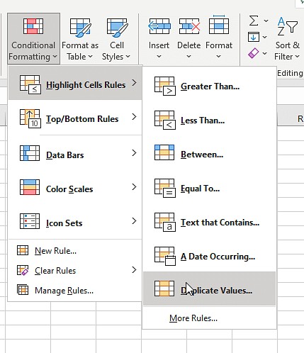
2. Go to the “Home” tab and click on “Conditional Formatting.”
3. Choose “Highlight Cells Rules” and select “Duplicate Values” to find matches, or “More Rules” to define custom criteria.
4. Customize the formatting style (e.g., cell color, font color) to highlight the desired cells.
5. Click “OK” to apply the conditional formatting.

Pros:

• Visually intuitive and easy to implement.
• Allows for quick identification of patterns and anomalies.
• Customizable formatting options.

Cons:

• Limited to visual highlighting; doesn’t provide numerical summaries or data extraction.
• May not be suitable for very large datasets due to performance considerations.

2.2 Equals Operator (=)

The equals operator provides a simple way to compare individual cells in two columns. By using a formula, you can determine whether corresponding cells contain the same value.

Steps:

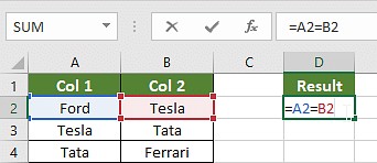
1. Create a new column next to the columns you want to compare.
2. In the first cell of the new column, enter the formula =A1=B1 (assuming the first values are in A1 and B1).
3. Drag the formula down to apply it to all rows.
4. The new column will display “TRUE” for matching cells and “FALSE” for non-matching cells.

Pros:

• Simple and straightforward.
• Provides a clear “TRUE” or “FALSE” result for each cell comparison.
• Can be combined with other functions for more complex logic.

Cons:

• Requires creating an additional column.
• Doesn’t provide summaries or visualizations.
• Case-sensitive; “Apple” and “apple” will be considered different.

2.3 IF Formula

The IF formula allows you to perform conditional comparisons and display custom messages based on the results. This method is useful for categorizing matches and differences.

Syntax:

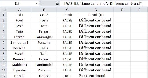
=IF(condition, value_if_true, value_if_false)

Example:

=IF(A1=B1, "Match", "Mismatch")

This formula compares the values in cells A1 and B1. If they are equal, it displays “Match”; otherwise, it displays “Mismatch.”

Pros:

• Allows for customized output messages.
• Flexible and adaptable to various comparison scenarios.
• Can be combined with other functions for more complex logic.

Cons:

• Requires creating an additional column.
• Can become complex for intricate comparison criteria.

2.4 VLOOKUP Function

The VLOOKUP function searches for a value in the first column of a table and returns a corresponding value from another column in the same table. This method is useful for finding matches and extracting related data.

Syntax:

=VLOOKUP(lookup_value, table_array, col_index_num, [range_lookup])

• lookup_value: The value you want to search for.
• table_array: The range of cells containing the data to search.
• col_index_num: The column number in the table_array from which to return the matching value.
• [range_lookup]: Optional. TRUE for approximate match, FALSE for exact match.

Example:

Assuming column A contains a list of IDs and column B contains corresponding names, to check if an ID in column C exists in column A and return the corresponding name:

=VLOOKUP(C1, A:B, 2, FALSE)

If the ID in C1 exists in column A, the formula returns the corresponding name from column B. If not, it returns an error.

Pros:

• Efficient for finding matches and extracting related data.
• Can handle large datasets.
• Useful for data validation and reconciliation.

Cons:

• Requires the lookup value to be in the first column of the table array.
• Returns an error if the lookup value is not found (can be handled with IFERROR).

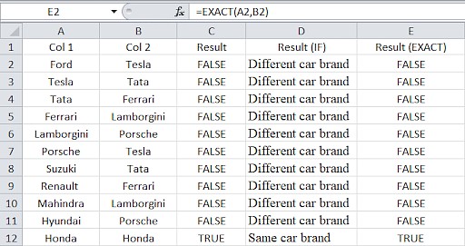
2.5 EXACT Formula

The EXACT formula compares two text strings and returns TRUE if they are exactly the same, including case. This method is useful for case-sensitive comparisons.

Syntax:

=EXACT(text1, text2)

Example:

=EXACT(A1, B1)

This formula compares the text in cells A1 and B1. It returns TRUE only if the text is identical, including case.

Pros:

• Case-sensitive comparison.
• Simple and straightforward.
• Useful for verifying data accuracy where case matters.

Cons:

• Limited to text comparisons.
• Doesn’t provide summaries or visualizations.

3. Choosing the Right Method

The best method for comparing two columns in Excel depends on your specific needs and the characteristics of your data. Here’s a guide to help you choose:

Method	Use Case	Pros	Cons
Conditional Formatting	Quickly identifying matches, differences, or duplicates visually.	Visually intuitive, easy to implement, customizable.	Limited to visual highlighting, may not be suitable for large datasets.
Equals Operator (=)	Simple cell-by-cell comparison with TRUE/FALSE results.	Simple, straightforward, can be combined with other functions.	Requires an additional column, no summaries, case-sensitive.
IF Formula	Categorizing matches and differences with custom messages.	Customizable output, flexible, can be combined with other functions.	Requires an additional column, can become complex for intricate criteria.
VLOOKUP Function	Finding matches and extracting related data from another table.	Efficient, can handle large datasets, useful for data validation.	Requires lookup value in the first column, returns an error if not found.
EXACT Formula	Case-sensitive comparison of text strings.	Case-sensitive, simple, useful for verifying data accuracy where case matters.	Limited to text comparisons, no summaries or visualizations.

4. Advanced Techniques for Column Comparison

Beyond the basic methods, Excel offers advanced techniques for more complex column comparison scenarios.

4.1 Comparing Multiple Columns

To compare multiple columns for row matches, you can use the AND and COUNTIF functions.

AND Function:

=IF(AND(A1=B1, A1=C1), "Complete Match", "")

This formula checks if the values in cells A1, B1, and C1 are all equal. If they are, it displays “Complete Match”; otherwise, it displays nothing.

COUNTIF Function:

=IF(COUNTIF($A1:$C1, $A1)=3, "Complete Match", "")

This formula counts how many times the value in cell A1 appears in the range A1:C1. If the count is equal to 3 (the number of columns), it means all three cells have the same value, and the formula displays “Complete Match.”

4.2 Finding Unique Values

To find unique values in one column that are not present in another, you can use the COUNTIF and ISERROR/MATCH functions.

COUNTIF Function:

=IF(COUNTIF($B:$B, $A1)=0, "Not in B", "")

This formula checks if the value in cell A1 exists in column B. If the count is 0, it means the value is not present in column B, and the formula displays “Not in B.”

ISERROR and MATCH Functions:

=IF(ISERROR(MATCH($A1, $B:$B, 0)), "Not in B", "")

This formula uses the MATCH function to search for the value in cell A1 in column B. If the MATCH function returns an error (meaning the value is not found), the ISERROR function returns TRUE, and the IF formula displays “Not in B.”

4.3 Comparing Two Lists and Pulling Matching Data

To compare two lists and extract matching data, you can use the VLOOKUP, INDEX/MATCH, or XLOOKUP functions.

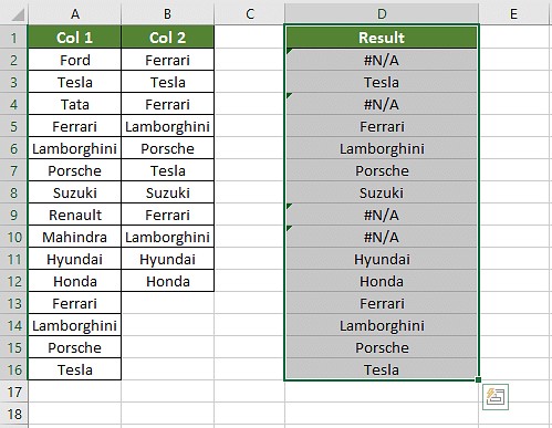
VLOOKUP Function:

=VLOOKUP(D1, $A:$B, 2, FALSE)

Assuming column A contains a list of IDs and column B contains corresponding names, and column D contains another list of IDs, this formula searches for the ID in cell D1 in column A and returns the corresponding name from column B.

INDEX and MATCH Functions:

=INDEX($B:$B, MATCH($D1, $A:$A, 0))

This formula uses the MATCH function to find the row number of the ID in cell D1 in column A. Then, it uses the INDEX function to return the value from column B in that row.

XLOOKUP Function (Excel 365 and later):

=XLOOKUP(D1, $A:$A, $B:$B)

This formula searches for the ID in cell D1 in column A and returns the corresponding value from column B. XLOOKUP is more flexible and easier to use than VLOOKUP and INDEX/MATCH.

5. Practical Examples of Column Comparison

Let’s explore some practical examples of how column comparison can be used in real-world scenarios.

5.1 Data Validation

Imagine you have two spreadsheets containing customer data. One spreadsheet is from your CRM system, and the other is from a marketing campaign. You want to ensure that all customers in the marketing campaign spreadsheet are also present in the CRM system.

You can use the VLOOKUP function to compare the customer IDs in the two spreadsheets. If the VLOOKUP function returns an error, it means the customer ID is not present in the CRM system.

5.2 Identifying Duplicates

Suppose you have a spreadsheet containing a list of email addresses. You want to identify any duplicate email addresses.

You can use conditional formatting to highlight duplicate email addresses. Select the column containing the email addresses, go to “Conditional Formatting,” choose “Highlight Cells Rules,” and select “Duplicate Values.”

5.3 Finding Discrepancies

Let’s say you have two spreadsheets containing sales data. One spreadsheet is from your sales team, and the other is from your accounting system. You want to find any discrepancies between the sales figures in the two spreadsheets.

You can use the IF formula to compare the sales figures in the two spreadsheets. If the IF formula returns “Mismatch,” it means there is a discrepancy between the sales figures.

6. Best Practices for Column Comparison

To ensure accurate and efficient column comparison, follow these best practices:

• Clean and Prepare Your Data: Before comparing columns, ensure that your data is clean and consistent. Remove any leading or trailing spaces, correct any spelling errors, and standardize data formats.
• Understand Your Data: Before comparing columns, take the time to understand your data. What do the columns represent? What are the possible values? Are there any known issues or inconsistencies?
• Choose the Right Method: Select the appropriate method for your specific needs and the characteristics of your data. Consider the size of your dataset, the type of comparison you need to perform, and the level of detail you require.
• Test Your Formulas: Before applying your formulas to the entire dataset, test them on a small sample to ensure that they are working correctly.
• Document Your Steps: Keep a record of the steps you take to compare columns. This will help you to reproduce your results and troubleshoot any issues.
• Use Comments: Add comments to your formulas to explain what they do. This will make it easier to understand your formulas later.
• Error Handling: Use error handling techniques to prevent your formulas from returning errors. For example, you can use the IFERROR function to display a custom message if a formula returns an error.

7. Common Mistakes to Avoid

Here are some common mistakes to avoid when comparing columns in Excel:

• Not Cleaning and Preparing Your Data: Failing to clean and prepare your data can lead to inaccurate results.
• Using the Wrong Method: Using the wrong method can lead to inaccurate results or make the comparison process more difficult.
• Not Testing Your Formulas: Not testing your formulas can lead to errors that are difficult to detect.
• Not Understanding Your Data: Not understanding your data can lead to misinterpretations of the results.
• Ignoring Case Sensitivity: Forgetting that some functions (e.g., EXACT) are case-sensitive can lead to inaccurate results.
• Not Using Absolute References: Not using absolute references when necessary can cause your formulas to return incorrect results when you copy them to other cells.

8. Optimizing Excel for Column Comparisons

To improve the performance of Excel when comparing large datasets, consider these optimization tips:

• Use Efficient Formulas: Some formulas are more efficient than others. For example, using INDEX/MATCH is generally faster than VLOOKUP.
• Avoid Volatile Functions: Volatile functions (e.g., NOW(), RAND()) recalculate every time the spreadsheet is changed, which can slow down performance.
• Use Named Ranges: Using named ranges can make your formulas easier to read and understand, and it can also improve performance.
• Turn Off Automatic Calculation: If you are working with a very large dataset, you can turn off automatic calculation to prevent Excel from recalculating every time you make a change.
• Use Excel Tables: Excel tables are more efficient than regular ranges.
• Close Unnecessary Workbooks: Having multiple workbooks open can slow down Excel’s performance.
• Upgrade Your Hardware: If you are working with very large datasets, you may need to upgrade your computer’s hardware (e.g., RAM, processor) to improve performance.

9. FAQs About Comparing Columns in Excel

1. How do I compare two columns in Excel and highlight the differences?

You can use conditional formatting with a formula to highlight differences. For example, select the columns, go to “Conditional Formatting,” choose “New Rule,” select “Use a formula to determine which cells to format,” and enter the formula =A1<>B1.

2. Can I compare two columns in Excel for partial matches?

Yes, you can use functions like SEARCH or FIND within an IF formula to check for partial matches. For example, =IF(ISNUMBER(SEARCH(A1,B1)),"Partial Match","No Match").

3. How do I compare two lists in Excel and find the missing values?

You can use the COUNTIF function to check if each value in one list exists in the other list. If the COUNTIF returns 0, the value is missing.

4. How do I compare two columns with different lengths in Excel?

You can use the IFERROR function to handle errors when comparing columns with different lengths. For example, when using VLOOKUP, wrap the formula in IFERROR to return a specific value if no match is found.

5. How can I compare two columns and return a value from a third column if there is a match?

You can use the VLOOKUP or INDEX/MATCH functions to return a value from a third column based on a match in the first two columns.

6. Is there a way to compare two columns in Excel without using formulas?

Yes, you can use the “Remove Duplicates” feature to find unique values in one column that are not present in the other.

7. How do I compare two columns in Excel and ignore case?

Use the UPPER or LOWER functions to convert both columns to the same case before comparing them. For example, =IF(UPPER(A1)=UPPER(B1),"Match","No Match").

8. Can I compare two columns in Excel using VBA?

Yes, you can use VBA to automate the comparison process and perform more complex tasks.

9. How do I compare two columns in Excel and highlight the entire row if there is a match?

Use conditional formatting with a formula that references the entire row. For example, select the entire range of data, go to “Conditional Formatting,” choose “New Rule,” select “Use a formula to determine which cells to format,” and enter the formula =$A1=$B1.

10. What is the best way to compare two columns in Excel for performance?

For large datasets, using INDEX/MATCH is generally faster than VLOOKUP. Also, avoid volatile functions and use named ranges to improve performance.

10. Simplify Data Comparison with COMPARE.EDU.VN

Comparing values in Excel can be time-consuming and complex, especially when dealing with large datasets or intricate comparison criteria. At COMPARE.EDU.VN, we understand these challenges and offer comprehensive solutions to streamline your data comparison process.

Our website provides detailed comparisons, tutorials, and tools to help you make informed decisions based on accurate and reliable data. Whether you’re comparing product features, service offerings, or educational programs, COMPARE.EDU.VN empowers you to analyze and evaluate your options effectively.

Ready to unlock the power of data-driven decision-making?

Visit COMPARE.EDU.VN today and explore our extensive collection of comparisons and resources.

Contact us:

• Address: 333 Comparison Plaza, Choice City, CA 90210, United States
• WhatsApp: +1 (626) 555-9090
• Website: COMPARE.EDU.VN

Let compare.edu.vn be your trusted partner in data comparison and informed decision-making. Make the right choice, every time.