How to Compare Values in 2 Columns in Excel

Comparing values in two columns in Excel can be a game-changer for data analysis, offering valuable insights for informed decision-making. At COMPARE.EDU.VN, we understand the importance of efficient data comparison and provide you with the tools and techniques to master this essential skill, making data analysis a breeze. Whether it’s identifying matching entries, pinpointing discrepancies, or extracting specific information, Excel offers a variety of methods to streamline the process.

1. Understanding the Need to Compare Values in Excel

Excel is a powerful tool for data management and analysis, widely used across various industries. One common task is comparing data between two or more columns. This could involve:

• Identifying duplicate entries
• Finding matching values across different datasets
• Highlighting discrepancies or differences
• Performing conditional calculations based on comparison results

Without the ability to effectively compare values, these tasks become time-consuming and prone to errors. Mastering Excel’s comparison techniques significantly enhances your data analysis capabilities.

2. Common Scenarios for Column Comparison in Excel

Let’s explore some practical scenarios where comparing values in Excel columns is essential:

• Sales Data Analysis: Comparing sales figures for different periods to identify growth or decline.
• Inventory Management: Matching stock levels between different warehouses to optimize distribution.
• Customer Relationship Management (CRM): Identifying duplicate customer entries to maintain data accuracy.
• Financial Analysis: Comparing budget figures against actual expenses to track financial performance.
• Research and Development: Comparing experimental results to identify statistically significant differences.

These examples highlight the versatility of Excel’s comparison capabilities across diverse fields.

3. Methods to Compare Values in Two Columns in Excel

Excel provides several methods to compare values in two columns, each with its own advantages and use cases. Let’s explore these methods in detail:

3.1 Conditional Formatting

Conditional formatting is a quick and visual way to highlight matching or differing values.

Steps:

1. Select the two columns you want to compare.
2. Go to the “Home” tab.
3. Click on “Conditional Formatting”.
4. Choose “Highlight Cells Rules”.
5. Select “Duplicate Values” to highlight matching entries or “More Rules” to define custom criteria.
6. Choose a formatting style (e.g., fill color, font color).
7. Click “OK”.

Example: Highlight all matching email addresses in two customer lists.

Advantages:

• Simple and intuitive to use
• Provides visual cues for quick identification

Disadvantages:

• Limited to highlighting, doesn’t provide specific results in a separate column
• Can be slow with large datasets

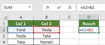
3.2 Using the Equals Operator (=)

The equals operator is a basic but effective way to compare values row by row.

Steps:

1. In a new column, enter the formula =A1=B1 (assuming your data starts in row 1).
2. Drag the formula down to apply it to all rows.
3. The formula will return TRUE if the values in columns A and B are equal, and FALSE otherwise.

Example: Checking if the product IDs in two inventory lists match for each item.

Advantages:

• Simple and direct
• Provides a clear TRUE/FALSE result

Disadvantages:

• Doesn’t provide additional information beyond the comparison result
• Can be cumbersome for large datasets

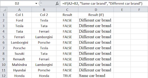
3.3 IF Formula

The IF formula allows you to perform different actions based on the comparison result.

Syntax: =IF(A1=B1, "Match", "No Match")

Steps:

1. In a new column, enter the IF formula.
2. Drag the formula down to apply it to all rows.
3. The formula will return “Match” if the values in columns A and B are equal, and “No Match” otherwise.

Example: Displaying “Same Product” or “Different Product” based on the product names in two columns.

Advantages:

• More flexible than the equals operator
• Allows for custom messages or calculations based on the comparison

Disadvantages:

• Can become complex with multiple conditions
• Requires careful attention to syntax

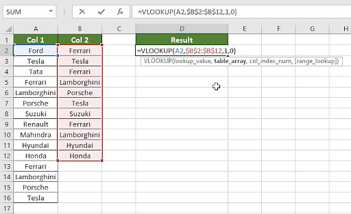
3.4 VLOOKUP Function

The VLOOKUP function is useful for finding matching values in one column based on another.

Syntax: =VLOOKUP(lookup_value, table_array, col_index_num, [range_lookup])

Steps:

1. In a new column, enter the VLOOKUP formula.
2. lookup_value: The value you want to find in the first column of the table array (e.g., A1).
3. table_array: The range of cells containing the data you want to search (e.g., B:B).
4. col_index_num: The column number in the table array from which you want to retrieve a value (usually 1).
5. [range_lookup]: FALSE for an exact match.
6. Drag the formula down to apply it to all rows.
7. If a match is found, VLOOKUP returns the corresponding value; otherwise, it returns #N/A.

Example: Finding the price of a product in a price list based on the product name in another column.

Advantages:

• Powerful for retrieving related data based on a match
• Can handle large datasets efficiently

Disadvantages:

• Can be complex to set up
• Returns #N/A for non-matches, which may require additional handling

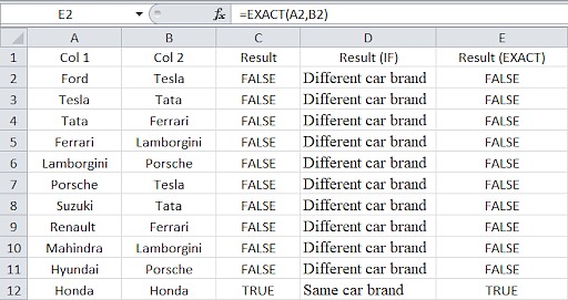
3.5 EXACT Function

The EXACT function compares two strings and returns TRUE only if they are exactly the same, including case.

Syntax: =EXACT(A1, B1)

Steps:

1. In a new column, enter the EXACT formula.
2. Drag the formula down to apply it to all rows.
3. The formula will return TRUE if the values in columns A and B are exactly the same (including case), and FALSE otherwise.

Example: Verifying if the usernames in two databases are identical, including capitalization.

Advantages:

• Case-sensitive comparison
• Useful for ensuring data integrity

Disadvantages:

• Strict comparison, may not be suitable for all scenarios
• Doesn’t provide additional information beyond the comparison result

4. Advanced Techniques for Complex Comparisons

For more complex scenarios, you can combine these basic techniques or use more advanced functions.

4.1 Combining IF and ISNA Functions

To handle the #N/A errors returned by VLOOKUP, you can use the ISNA function within an IF formula.

Syntax: =IF(ISNA(VLOOKUP(A1, B:B, 1, FALSE)), "Not Found", "Found")

This formula will return “Not Found” if the VLOOKUP returns #N/A, and “Found” otherwise.

4.2 Using INDEX and MATCH Functions

The INDEX and MATCH functions can be used together as a more flexible alternative to VLOOKUP.

Syntax: =INDEX(B:B, MATCH(A1, A:A, 0))

This formula will return the value from column B that corresponds to the row where A1 is found in column A.

4.3 Using COUNTIF Function

The COUNTIF function counts the number of cells within a range that meet a given criteria.

Syntax: =COUNTIF(B:B, A1)

This formula will return the number of times the value in A1 appears in column B. A result greater than 0 indicates a match.

5. Choosing the Right Method

The best method for comparing columns in Excel depends on your specific needs. Here’s a summary to help you choose:

Method	Use Case	Advantages	Disadvantages
Conditional Formatting	Visualizing matches or differences quickly	Simple, intuitive, visual cues	Limited functionality, slow with large datasets
Equals Operator	Simple row-by-row comparison	Simple, direct, clear TRUE/FALSE result	Limited functionality, cumbersome for large datasets
IF Formula	Performing different actions based on comparison results	Flexible, allows custom messages/calculations	Can be complex, requires careful syntax
VLOOKUP Function	Retrieving related data based on a match	Powerful, efficient with large datasets	Can be complex, returns #N/A for non-matches
EXACT Function	Case-sensitive comparison	Ensures data integrity, case-sensitive	Strict comparison, limited functionality
IF & ISNA Combination	Handling #N/A errors from VLOOKUP	More robust error handling	More complex syntax
INDEX & MATCH	Flexible alternative to VLOOKUP	More flexible, can handle more complex lookups	More complex syntax
COUNTIF	Counting occurrences of a value in another column	Simple for checking existence of values	Doesn’t retrieve related data

6. Real-World Examples

Let’s illustrate these methods with real-world examples.

6.1 Comparing Sales Data

Imagine you have two spreadsheets containing sales data for different months. You want to identify which products have increased in sales.

1. Column A: Product Name (Month 1)
2. Column B: Sales Quantity (Month 1)
3. Column C: Product Name (Month 2)
4. Column D: Sales Quantity (Month 2)

You can use the following steps:

1. Insert a new column E and use VLOOKUP to find the sales quantity from Month 1 for each product in Month 2:
   =VLOOKUP(C1, A:B, 2, FALSE)
2. Handle #N/A errors with IF and ISNA:
   =IF(ISNA(VLOOKUP(C1, A:B, 2, FALSE)), 0, VLOOKUP(C1, A:B, 2, FALSE))
3. Insert a new column F and calculate the sales difference:
   =D1 - E1
4. Use conditional formatting to highlight products with increased sales (positive difference).

6.2 Managing Inventory

You have two lists of inventory items from different warehouses. You want to identify items that are present in both warehouses.

1. Column A: Item ID (Warehouse 1)
2. Column B: Item Name (Warehouse 1)
3. Column C: Item ID (Warehouse 2)

You can use the following steps:

1. Insert a new column D and use COUNTIF to check if each item ID from Warehouse 1 exists in Warehouse 2:
   =COUNTIF(C:C, A1)
2. Use conditional formatting to highlight items present in both warehouses (COUNTIF result > 0).

6.3 Cleaning Customer Data

You have a list of customer names and email addresses. You want to identify and remove duplicate entries.

1. Column A: Customer Name
2. Column B: Email Address

You can use the following steps:

1. Select both columns and use conditional formatting to highlight duplicate values in the email address column.
2. Manually review the highlighted entries and remove duplicates.

7. Tips and Best Practices

• Ensure Data Consistency: Before comparing, ensure that the data in both columns is consistent in terms of format, case, and spelling.
• Use Helper Columns: Don’t hesitate to create additional columns to simplify your formulas and make them more readable.
• Test Your Formulas: Always test your formulas on a small sample of data before applying them to the entire dataset.
• Use Named Ranges: For complex formulas, consider using named ranges to make your formulas more understandable and maintainable.
• Document Your Work: Add comments to your formulas to explain their purpose and logic.
• Leverage Excel Tables: Convert your data ranges into Excel tables to take advantage of automatic formula propagation and structured references.

8. Troubleshooting Common Issues

• #N/A Errors: These errors typically occur when VLOOKUP or MATCH can’t find a match. Use the ISNA function to handle these errors gracefully.
• Incorrect Results: Double-check your formulas and ensure that the ranges and column indices are correct.
• Slow Performance: For large datasets, consider using array formulas or Power Query to improve performance.
• Case Sensitivity: Remember that the EXACT function is case-sensitive. Use the UPPER or LOWER functions to convert data to a consistent case before comparing.
• Format Inconsistencies: Ensure that the data in both columns is formatted consistently. Use the TEXT function to convert numbers to text or vice versa.

9. Beyond the Basics: Advanced Excel Features for Comparison

Excel offers several advanced features that can further enhance your comparison capabilities.

9.1 Power Query

Power Query is a powerful data transformation and manipulation tool that can be used to compare data from multiple sources, clean and transform data, and perform complex joins and aggregations.

9.2 Array Formulas

Array formulas allow you to perform calculations on multiple values at once. They can be used to compare entire ranges of data with a single formula.

9.3 Pivot Tables

Pivot tables are a powerful tool for summarizing and analyzing data. They can be used to compare data across different categories and dimensions.

9.4 Macros (VBA)

For highly customized or repetitive comparison tasks, you can use VBA macros to automate the process.

10. Utilizing COMPARE.EDU.VN for Comprehensive Comparisons

While Excel offers powerful tools for comparing values, sometimes you need a more comprehensive and structured approach. That’s where COMPARE.EDU.VN comes in.

COMPARE.EDU.VN provides detailed comparisons across various categories, including:

• Products: Compare features, specifications, prices, and reviews of different products.
• Services: Evaluate different service providers based on their offerings, pricing, and customer feedback.
• Ideas: Explore different concepts and approaches to make informed decisions.

By leveraging COMPARE.EDU.VN, you can:

• Gain a broader perspective: See how different options stack up against each other.
• Save time and effort: Avoid spending hours researching and comparing data manually.
• Make informed decisions: Base your choices on comprehensive and objective comparisons.

11. FAQs about Comparing Values in Excel

Here are some frequently asked questions about comparing values in Excel:

1. How do I compare two columns for duplicates and highlight them?

Use conditional formatting with the “Duplicate Values” rule. Select the columns, go to Home > Conditional Formatting > Highlight Cells Rules > Duplicate Values.

2. Can I compare two columns in different Excel files?

Yes, but you need to reference the other file in your formulas. For example, =[OtherFile.xlsx]Sheet1!A1 refers to cell A1 in Sheet1 of OtherFile.xlsx.

3. How do I ignore case when comparing two columns?

Use the UPPER or LOWER functions to convert the data to a consistent case before comparing. For example, =UPPER(A1)=UPPER(B1).

4. How do I compare two columns and return a value from a third column?

Use VLOOKUP or INDEX/MATCH. For example, if you want to return the value from column C when A1 matches a value in column B, use =VLOOKUP(A1, B:C, 2, FALSE).

5. How do I compare two columns and highlight the entire row if there’s a match?

Use conditional formatting with a formula. Select the entire data range, go to Home > Conditional Formatting > New Rule > Use a formula to determine which cells to format. Enter the formula =A1=B1 and choose a formatting style.

6. How do I compare two columns and extract the unique values from each?

Use the Advanced Filter feature with the “Unique records only” option. Select the column, go to Data > Advanced Filter, choose “Copy to another location”, select the range, check “Unique records only”, and specify the copy location.

7. How do I compare two columns and count the number of matches?

Use the SUMPRODUCT function. For example, =SUMPRODUCT(--(A1:A10=B1:B10)) will count the number of rows where the values in columns A and B match.

8. How do I compare two columns and find the first difference?

Use a combination of IF and ROW functions. Enter the formula =IF(A1<>B1, ROW(), "") in a new column, drag it down, and then find the smallest row number in that column.

9. How do I compare two columns and create a new column with the differences?

Use an IF formula. For example, =IF(A1=B1, "", A1&" vs " &B1) will return an empty string if the values match, and a string with the differences otherwise.

10. How can I compare two columns and get the percentage match?

• Step 1: Determine the total number of rows to be evaluated.
• Step 2: Use the formula =SUMPRODUCT(–(A1:A10=B1:B10)) to get the number of matching rows.
• Step 3: Divide the result in step 2 by the result in step 1 and format it as a percentage.

12. Conclusion: Empowering Your Data Analysis with Excel and COMPARE.EDU.VN

Mastering the techniques for comparing values in Excel columns is a valuable skill for anyone working with data. By understanding the different methods and their applications, you can streamline your data analysis tasks and gain deeper insights. Remember to leverage the power of COMPARE.EDU.VN for comprehensive comparisons and informed decision-making.

Ready to take your data analysis skills to the next level? Visit COMPARE.EDU.VN today to explore detailed comparisons across various categories and make confident choices. Whether you’re comparing products, services, or ideas, COMPARE.EDU.VN is your go-to resource for objective and comprehensive information.

Don’t just compare, COMPARE.EDU.VN!

For further assistance or inquiries, please contact us at:

• Address: 333 Comparison Plaza, Choice City, CA 90210, United States
• WhatsApp: +1 (626) 555-9090
• Website: compare.edu.vn