How to Compare Two Worksheets in Excel Using VLOOKUP

Comparing data across multiple spreadsheets can be a tedious task. Fortunately, Excel’s VLOOKUP function provides a powerful solution for efficiently comparing two worksheets and identifying discrepancies. This article outlines a step-by-step guide on how to leverage VLOOKUP to compare two Excel worksheets, reconcile data, and highlight differences.

Setting Up Your Data for Comparison

The first step involves organizing your data in a way that facilitates comparison. Begin by copying the data from both sources into two separate sheets within the same Excel workbook. Ensure that both worksheets have identical column headers, even if the data within those columns differs. A unique identifier column, such as “Customer ID” or “Invoice Number,” is crucial for this process.

Utilizing VLOOKUP for Data Matching

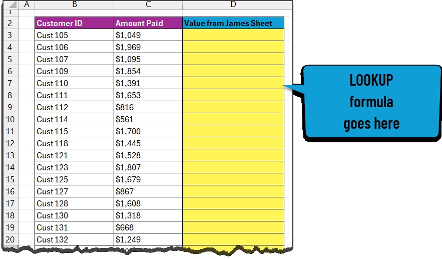
With your data prepared, navigate to the first worksheet. In a new column adjacent to your data, you’ll insert the VLOOKUP formula. This formula will search for matching values in the second worksheet based on the unique identifier.

The general syntax of the VLOOKUP formula is:

=VLOOKUP(lookup_value, table_array, col_index_num, [range_lookup])

In this context:

• lookup_value: The cell containing the unique identifier in the first sheet (e.g., Customer ID).
• table_array: The range of cells in the second sheet containing the data you want to compare, including the unique identifier column and the column you want to retrieve. Important: Use absolute references (e.g., $B$3:$C$32) to ensure the range remains fixed when copying the formula.
• col_index_num: The column number within table_array from which to retrieve the matching value.
• [range_lookup]: Set to FALSE for exact matches.

For example: =VLOOKUP(B3,'Sheet2'!$B$3:$C$32,2,FALSE) This formula searches for the value in cell B3 of the first sheet within column B of Sheet2 (range $B$3:$C$32) and returns the corresponding value from the second column (column C) of Sheet2.

Copy this formula down the entire column to retrieve matching values for all unique identifiers.

Using XLOOKUP (Excel 365 and later)

If you’re using Excel 365 or later versions, XLOOKUP offers a more flexible alternative:

=XLOOKUP(B3,'Sheet2'!$B$3:$B$32,'Sheet2'!$C$3:$C$32,"ID missing") 

This formula performs the same function as VLOOKUP but with enhanced error handling (returning “ID missing” if no match is found).

Reconciling and Identifying Discrepancies

After retrieving matching values, you can use the IF function to identify differences:

=IF(ISERROR(D3),"ID Missing", IF(D3<>C3,"Not matching", "Matching"))

This formula checks for three scenarios:

1. “ID Missing”: If VLOOKUP/XLOOKUP returns an error (e.g., #N/A), indicating the ID is not found in the second sheet.
   
2. “Not matching”: If the values in the two sheets are different.
3. “Matching”: If the values in the two sheets are identical.

Highlighting Differences with Conditional Formatting

To visually highlight discrepancies, apply conditional formatting:

1. Select the data range.
2. Go to Home > Conditional Formatting > New Rule…
3. Choose “Use a formula to determine which cells to format.”
4. Enter the formula =$E3="Not matching" for highlighting non-matching values and create a separate rule with =$E3="ID Missing" for missing IDs. Choose a distinct formatting style for each rule.

Conclusion

VLOOKUP and XLOOKUP offer a robust method for comparing two Excel worksheets. This approach empowers you to quickly identify missing IDs, reconcile data discrepancies, and gain valuable insights by highlighting differences with conditional formatting. Mastering this technique will significantly enhance your data analysis capabilities in Excel.