Comparing slopes is crucial in linear regression analysis to understand how relationships between variables differ under various conditions. This involves determining if the rate of change (slope) between an independent variable (X) and a dependent variable (Y) significantly changes across different groups or scenarios. This article outlines how to compare slopes effectively.
Understanding Slope Comparison
Imagine analyzing the relationship between advertising spend (X) and sales revenue (Y) for two different marketing campaigns. Comparing the slopes of the regression lines for each campaign reveals whether the effectiveness of advertising spend differs between them. A steeper slope indicates a stronger positive relationship, meaning that each dollar spent on advertising generates more revenue.
Visually inspecting graphed regression lines can provide an initial assessment. However, statistical tests are necessary to confirm if observed differences are statistically significant or merely due to random chance.
Performing Slope Comparison Using Regression Analysis
A common approach to compare slopes involves using a multiple linear regression model with an interaction term. Here’s a breakdown of the process:
1. Data Preparation:
- Categorical Variable: Introduce a categorical variable representing the different groups or conditions being compared (e.g., “Campaign A” and “Campaign B” in the advertising example).
- Interaction Term: Create an interaction term by multiplying the independent variable (X) by the categorical variable. This term captures how the relationship between X and Y changes depending on the group.
2. Model Building:
- Fit the Model: Use statistical software to fit a multiple linear regression model including the independent variable (X), the categorical variable, and the interaction term as predictors.
3. Interpreting Results:
- Coefficient of the Interaction Term: The coefficient of the interaction term indicates the difference in slopes between the groups. A statistically significant (p-value < 0.05) positive coefficient suggests that the slope is steeper for one group compared to the other. A negative coefficient suggests the opposite.
- Visual Inspection: Plot the regression lines for each group on a scatter plot. This visual representation aids in understanding the magnitude and direction of the slope differences.
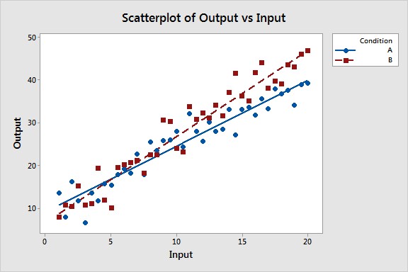 Scatterplot with two regression lines representing different slopes.
Example: Comparing Slopes of Height and Weight
Consider comparing the relationship between height (X) and weight (Y) for athletes and non-athletes.
- Categorical Variable: Create a variable “Athlete” with values of 1 for athletes and 0 for non-athletes.
- Interaction Term: Calculate “Height*Athlete.”
- Regression Model: Weight = β0 + β1(Height) + β2(Athlete) + β3(Height*Athlete)
- Interpretation: If β3 is statistically significant and positive, it implies that the slope of the height-weight relationship is steeper for athletes, suggesting that for every inch increase in height, athletes gain more weight on average compared to non-athletes.
Conclusion
Comparing slopes allows for a deeper understanding of how relationships between variables vary across different groups or conditions. Utilizing regression analysis with an interaction term provides a robust statistical method for quantifying and testing these differences, leading to more informed conclusions. Always remember to consider both the statistical significance and the practical significance of the slope differences in the context of your specific analysis.