How to Compare Two Sheets in Excel for Matches

Finding matching data across multiple Excel spreadsheets can be tedious. Fortunately, Excel offers powerful features to automate this process. This guide provides a step-by-step approach to efficiently compare two Excel sheets for matches using formulas and conditional formatting.

Comparing Data with the MATCH Function

The MATCH function is a core tool for identifying matching values. It returns the relative position of a value within a range. Here’s how to utilize it:

1. Prepare Your Worksheets: Ensure both sheets reside within the same workbook.

2. Designate a Helper Column: Choose a column in one sheet to display the results of the comparison.

3. Implement the MATCH Formula: In the helper column’s first cell, enter the following formula:

   =MATCH(lookup_value, lookup_array, match_type)

   • lookup_value: The cell containing the value you want to find in the other sheet. For instance, if you’re comparing values in column B, starting with row 2, this would be B2.

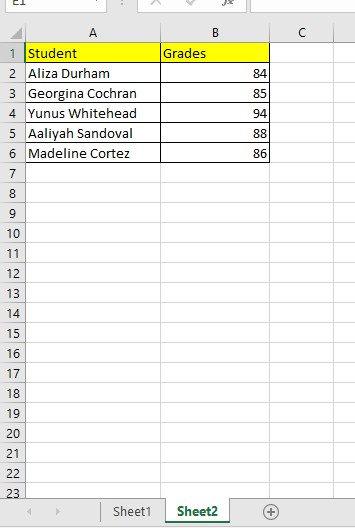
   • lookup_array: The range in the second sheet where you want to search for the lookup_value. For example, to search column B from rows 2 to 6 in Sheet1, use Sheet1!B2:B6. Using absolute references ($) will ensure the range remains constant when copying the formula down.

   • match_type: Set to 0 for an exact match.

   Example: =MATCH(B2,Sheet1!$B$2:$B$6,0)

4. Interpret Results: The formula returns a number indicating the position of the match in the lookup_array. If no match is found, it returns #N/A.

Highlighting Matches with Conditional Formatting

To visually emphasize matching data, leverage conditional formatting:

1. Select Data: Choose the column in the first sheet containing the values you want to highlight.

2. Apply Conditional Formatting: Go to Home > Conditional Formatting > Highlight Cells Rules > Equal To.

3. Configure the Rule: In the dialog box, use a formula to determine which cells to format. Enter the following formula:
   =ISNUMBER(MATCH(B2,Sheet1!$B$2:$B$6,0))

Choose a formatting style to highlight the matched cells.

4. Review Highlighted Cells: Matched data will now be visually distinct.

Conclusion

Comparing two Excel sheets for matches is simplified with the MATCH function and conditional formatting. These tools enable efficient data analysis and identification of corresponding entries across spreadsheets. By mastering these techniques, you can streamline your workflow and gain valuable insights from your data.