How To Compare Two Sheets Data In Excel

Comparing data across two Excel sheets can be a daunting task, but it’s essential for data reconciliation and analysis; COMPARE.EDU.VN offers a streamlined solution. This guide will walk you through a comprehensive, step-by-step process, exploring various Excel features and techniques to compare and reconcile data, ensuring accuracy and efficiency.

1. Understanding the Need to Compare Excel Sheets

Comparing data between two Excel sheets is a common task across various industries and roles. It’s essential for identifying discrepancies, ensuring data accuracy, and making informed decisions. Whether you’re reconciling financial statements, comparing sales data, or validating customer information, the ability to efficiently compare Excel sheets is a valuable skill. Let’s delve into the reasons and scenarios where this becomes crucial, highlighting the advantages of utilizing COMPARE.EDU.VN for streamlined solutions and efficient data comparison techniques.

1.1. Reasons for Comparing Excel Sheets

Data Validation: Ensuring that data entered into one sheet matches the data in another, especially after manual entry or data migration.
Reconciliation: Matching records between two datasets to identify discrepancies, such as in accounting or inventory management.
Change Tracking: Identifying what has changed between two versions of a spreadsheet, useful for version control and auditing.
Data Analysis: Comparing trends and patterns across different datasets to gain insights and make informed decisions.
Reporting: Consolidating data from multiple sources into a single report, requiring a comparison to avoid duplication or inconsistencies.

1.2. Scenarios Where Comparison Is Essential

Financial Audits: Comparing financial records from different departments or systems to ensure accuracy and compliance.
Sales Analysis: Comparing sales data from different periods or regions to identify trends and performance issues.
Inventory Management: Comparing inventory records with actual stock levels to identify discrepancies and prevent losses.
Customer Relationship Management (CRM): Comparing customer data from different sources to create a unified view and improve customer service.
Project Management: Comparing project plans with actual progress to identify delays and resource allocation issues.

1.3. Challenges in Comparing Excel Sheets

While comparing Excel sheets is essential, it can be challenging, especially with large datasets. Some common challenges include:

Large Datasets: Manually comparing thousands of rows and columns is time-consuming and prone to errors.
Different Formats: Data may be stored in different formats, making it difficult to compare directly.
Inconsistent Data Entry: Variations in data entry, such as spelling errors or inconsistent capitalization, can lead to mismatches.
Complex Formulas: Comparing sheets with complex formulas can be challenging, as changes in one sheet may affect multiple cells in another.
Data Security: Sharing sensitive data between different users or systems can raise security concerns.

1.4. How COMPARE.EDU.VN Helps

COMPARE.EDU.VN offers a range of tools and resources to help you overcome these challenges and efficiently compare Excel sheets. Our platform provides:

Step-by-Step Guides: Detailed tutorials on various Excel comparison techniques, including VLOOKUP, MATCH, INDEX, and conditional formatting.
Template Downloads: Ready-to-use templates for common comparison scenarios, such as reconciliation and change tracking.
Expert Advice: Access to experienced Excel users who can provide guidance and support.
Community Forum: A platform to connect with other Excel users and share tips and tricks.
Custom Solutions: Tailored solutions for complex comparison scenarios, including data integration and automation.

By leveraging COMPARE.EDU.VN, you can streamline your Excel comparison tasks, reduce errors, and make better-informed decisions. Let’s move on to exploring various techniques to compare data effectively.

2. Preparing Your Data for Comparison

Before diving into the comparison process, it’s crucial to prepare your data to ensure accuracy and efficiency. This involves cleaning, formatting, and organizing your data to make it easier to compare. Let’s explore the essential steps in data preparation, emphasizing the value of COMPARE.EDU.VN in offering guidance and resources for effective data cleansing.

2.1. Data Cleaning

Data cleaning is the process of identifying and correcting errors, inconsistencies, and inaccuracies in your data. This is a critical step, as unclean data can lead to misleading comparison results. Common data cleaning tasks include:

Removing Duplicates: Identifying and removing duplicate rows or records.
Correcting Spelling Errors: Fixing spelling mistakes and typos.
Standardizing Formatting: Ensuring that data is consistently formatted (e.g., dates, numbers, text).
Handling Missing Values: Deciding how to handle missing or null values (e.g., replacing with a default value, removing the row).
Removing Unnecessary Characters: Removing extra spaces, special characters, or HTML tags.

2.2. Data Formatting

Data formatting involves structuring your data to make it easier to compare. This may include:

Sorting: Sorting your data by a common field (e.g., customer ID, date) to make it easier to match records.
Filtering: Filtering your data to focus on specific subsets of records.
Creating Unique Identifiers: Creating a unique identifier column by combining multiple fields (e.g., customer name and address).
Transposing Data: Transposing rows and columns to make it easier to compare data in different orientations.
Splitting Columns: Splitting a single column into multiple columns to separate data elements (e.g., splitting a full name into first name and last name).

2.3. Data Organization

Data organization involves structuring your data to make it easier to compare. This may include:

Creating Tables: Converting your data into Excel tables to take advantage of features like structured references and automatic filtering.
Naming Ranges: Naming ranges of cells to make it easier to refer to them in formulas.
Using Headers: Ensuring that each column has a clear and descriptive header.
Freezing Panes: Freezing the top row or left column to keep headers visible when scrolling through large datasets.
Grouping and Ungrouping: Grouping related rows or columns to make it easier to navigate and compare data.

2.4. COMPARE.EDU.VN Resources for Data Preparation

COMPARE.EDU.VN offers a range of resources to help you prepare your data for comparison, including:

Data Cleaning Guides: Step-by-step tutorials on common data cleaning tasks.
Data Formatting Tips: Tips and tricks for formatting your data to make it easier to compare.
Data Organization Strategies: Strategies for organizing your data to make it easier to analyze and compare.
Template Downloads: Ready-to-use templates for data cleaning, formatting, and organization.
Expert Advice: Access to experienced Excel users who can provide guidance and support.

By following these data preparation steps and leveraging COMPARE.EDU.VN resources, you can ensure that your data is clean, formatted, and organized, leading to more accurate and efficient comparisons. Let’s proceed by exploring the core Excel functions for comparing data between sheets.

3. Using VLOOKUP to Compare Data

VLOOKUP (Vertical Lookup) is a powerful Excel function that allows you to search for a value in one column and return a corresponding value from another column in the same row. It’s a valuable tool for comparing data between two Excel sheets, especially when you have a common identifier. Let’s explore how to use VLOOKUP effectively for data comparison, emphasizing the resources provided by COMPARE.EDU.VN to master this function.

3.1. Understanding VLOOKUP Syntax

The syntax for VLOOKUP is as follows:

=VLOOKUP(lookup_value, table_array, col_index_num, [range_lookup])

lookup_value: The value you want to search for in the first column of the table array.
table_array: The range of cells that contains the data you want to search in.
col_index_num: The column number in the table array that contains the value you want to return.
range_lookup: An optional argument that specifies whether you want to find an exact match (FALSE) or an approximate match (TRUE).

3.2. Steps to Compare Data Using VLOOKUP

Identify a Common Identifier: Choose a column that exists in both sheets and contains unique values (e.g., customer ID, product code).
Open the First Sheet: Open the Excel sheet that you want to use as the primary source of data.
Insert a New Column: Insert a new column next to the column containing the common identifier. This column will hold the results of the VLOOKUP function.
Enter the VLOOKUP Formula: In the first cell of the new column, enter the VLOOKUP formula. For example:
```
=VLOOKUP(A2,'Sheet2'!A:B,2,FALSE)
```
- A2: The cell containing the lookup value in the first sheet.
- ‘Sheet2’!A:B: The table array in the second sheet (adjust the range as needed).
- 2: The column number in the second sheet that contains the value you want to return.
- FALSE: Specifies that you want to find an exact match.
Copy the Formula: Copy the formula down to all the rows in the column.
Interpret the Results:
- If VLOOKUP finds a matching value, it will return the corresponding value from the second sheet.
- If VLOOKUP does not find a matching value, it will return an #N/A error.
Handle #N/A Errors: Use the IFERROR function to handle #N/A errors. For example:
```
=IFERROR(VLOOKUP(A2,'Sheet2'!A:B,2,FALSE),"Not Found")
```
This formula will return “Not Found” if VLOOKUP does not find a matching value.

3.3. VLOOKUP Example

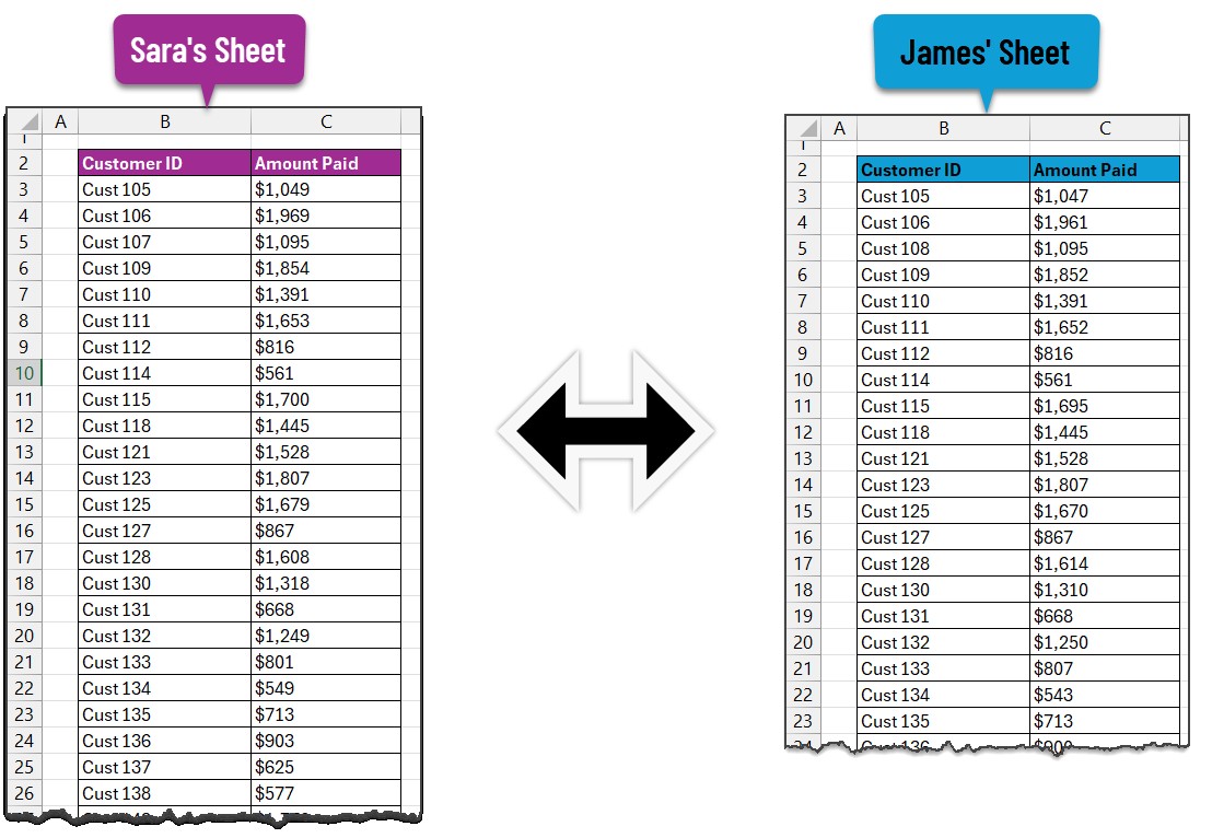
Let’s say you have two Excel sheets containing customer data. The first sheet contains customer IDs and names, while the second sheet contains customer IDs and email addresses. You want to compare the two sheets and find the email addresses for customers in the first sheet.

Common Identifier: Customer ID
First Sheet: Contains customer IDs and names
Second Sheet: Contains customer IDs and email addresses
VLOOKUP Formula:
```
=VLOOKUP(A2,'Sheet2'!A:B,2,FALSE)
```
- A2: The cell containing the customer ID in the first sheet.
- ‘Sheet2’!A:B: The table array in the second sheet (customer ID and email address columns).
- 2: The column number in the second sheet that contains the email address.
- FALSE: Specifies that you want to find an exact match.

3.4. COMPARE.EDU.VN Resources for VLOOKUP

COMPARE.EDU.VN provides a wealth of resources to help you master VLOOKUP, including:

VLOOKUP Tutorial: A comprehensive tutorial on how to use VLOOKUP, including examples and tips.
VLOOKUP Template: A ready-to-use template for comparing data using VLOOKUP.
VLOOKUP Examples: Real-world examples of how to use VLOOKUP in different scenarios.
VLOOKUP Troubleshooting: Tips for troubleshooting common VLOOKUP errors.
Expert Advice: Access to experienced Excel users who can provide guidance and support.

4. Using MATCH and INDEX for Advanced Comparisons

While VLOOKUP is a powerful tool, it has limitations. For example, it can only search for values in the first column of the table array and can be slow with large datasets. MATCH and INDEX offer more flexibility and performance for advanced comparisons. Let’s explore how to use MATCH and INDEX effectively for data comparison, highlighting the resources provided by COMPARE.EDU.VN to master these functions.

4.1. Understanding MATCH Syntax

The MATCH function searches for a specified item in a range of cells and returns the relative position of that item in the range. The syntax for MATCH is as follows:

=MATCH(lookup_value, lookup_array, [match_type])

lookup_value: The value you want to search for in the lookup array.
lookup_array: The range of cells that contains the data you want to search in.
match_type: An optional argument that specifies how you want to match the lookup value:
- 1: Finds the largest value that is less than or equal to the lookup value (lookup array must be sorted in ascending order).
- 0: Finds the first value that is exactly equal to the lookup value.
- -1: Finds the smallest value that is greater than or equal to the lookup value (lookup array must be sorted in descending order).

4.2. Understanding INDEX Syntax

The INDEX function returns the value of a cell in a table or range, based on its row and column number. The syntax for INDEX is as follows:

=INDEX(array, row_num, [column_num])

array: The range of cells that contains the data you want to retrieve.
row_num: The row number in the array that contains the value you want to retrieve.
column_num: An optional argument that specifies the column number in the array that contains the value you want to retrieve.

4.3. Combining MATCH and INDEX for Data Comparison

By combining MATCH and INDEX, you can overcome the limitations of VLOOKUP and perform more advanced data comparisons. Here’s how:

Use MATCH to Find the Row Number: Use the MATCH function to find the row number of the lookup value in the second sheet.
Use INDEX to Retrieve the Corresponding Value: Use the INDEX function to retrieve the corresponding value from the second sheet, based on the row number returned by MATCH.

4.4. MATCH and INDEX Example

Let’s revisit the customer data example from the VLOOKUP section. You have two Excel sheets containing customer data. The first sheet contains customer IDs and names, while the second sheet contains customer IDs and email addresses. You want to compare the two sheets and find the email addresses for customers in the first sheet, using MATCH and INDEX.

First Sheet: Contains customer IDs in column A and names in column B.
Second Sheet: Contains customer IDs in column A and email addresses in column B.
MATCH Formula: In the first sheet, use the MATCH function to find the row number of the customer ID in the second sheet.
```
=MATCH(A2,'Sheet2'!A:A,0)
```
- A2: The cell containing the customer ID in the first sheet.
- ‘Sheet2’!A:A: The range of cells containing the customer IDs in the second sheet.
- 0: Specifies that you want to find an exact match.
INDEX Formula: Use the INDEX function to retrieve the email address from the second sheet, based on the row number returned by MATCH.
```
=INDEX('Sheet2'!B:B,MATCH(A2,'Sheet2'!A:A,0))
```
- ‘Sheet2’!B:B: The range of cells containing the email addresses in the second sheet.
- MATCH(A2,’Sheet2′!A:A,0): The MATCH function returns the row number of the customer ID in the second sheet.

4.5. Advantages of Using MATCH and INDEX

Flexibility: MATCH and INDEX can search for values in any column, not just the first column.
Performance: MATCH and INDEX can be faster than VLOOKUP with large datasets.
Dynamic Ranges: MATCH and INDEX can handle dynamic ranges that change size.

4.6. COMPARE.EDU.VN Resources for MATCH and INDEX

COMPARE.EDU.VN offers a range of resources to help you master MATCH and INDEX, including:

MATCH Tutorial: A comprehensive tutorial on how to use MATCH, including examples and tips.
INDEX Tutorial: A comprehensive tutorial on how to use INDEX, including examples and tips.
MATCH and INDEX Examples: Real-world examples of how to use MATCH and INDEX in different scenarios.
MATCH and INDEX Troubleshooting: Tips for troubleshooting common MATCH and INDEX errors.
Expert Advice: Access to experienced Excel users who can provide guidance and support.

5. Using Conditional Formatting to Highlight Differences

Conditional formatting is a powerful Excel feature that allows you to automatically format cells based on certain criteria. It’s a valuable tool for highlighting differences between two Excel sheets, making it easier to identify discrepancies and patterns. Let’s explore how to use conditional formatting effectively for data comparison, emphasizing the resources provided by COMPARE.EDU.VN to enhance your data analysis skills.

5.1. Understanding Conditional Formatting Rules

Conditional formatting rules are based on formulas or criteria that you define. When a cell meets the criteria, the specified formatting is applied. Common conditional formatting rules include:

Highlight Cells Rules: Highlight cells that are greater than, less than, equal to, or between certain values.
Top/Bottom Rules: Highlight the top or bottom values in a range of cells.
Data Bars: Display data bars in cells to visualize the relative values.
Color Scales: Apply a color gradient to cells based on their values.
Icon Sets: Display icons in cells to represent different categories of values.
New Rule: Create custom rules based on formulas or criteria.

5.2. Steps to Compare Data Using Conditional Formatting

Select the Range of Cells: Select the range of cells that you want to compare.
Open Conditional Formatting: Go to the Home tab, click on Conditional Formatting, and choose a rule type.
Define the Rule Criteria: Define the criteria for the rule. This may involve entering a value, selecting a range of cells, or writing a formula.
Choose the Formatting: Choose the formatting that you want to apply when the rule is met. This may involve changing the font color, background color, or adding a border.
Apply the Rule: Click OK to apply the rule.

5.3. Conditional Formatting Example

Let’s say you have two Excel sheets containing sales data. The first sheet contains sales data for January, while the second sheet contains sales data for February. You want to compare the two sheets and highlight the cells where the sales data has changed significantly.

First Sheet: January sales data in column B.
Second Sheet: February sales data in column B.
Select the Range: Select the range of cells containing the sales data in both sheets (e.g., B2:B100 in both sheets).
Conditional Formatting: Go to Home > Conditional Formatting > New Rule.
Rule Type: Select “Use a formula to determine which cells to format”.
Formula: Enter the following formula to highlight cells where the sales data has increased by more than 10%:
```
=(B2-'Sheet1'!B2)/'Sheet1'!B2>0.1
```
- B2: The first cell in the selected range in the second sheet (February data).
- ‘Sheet1’!B2: The corresponding cell in the first sheet (January data).
- This formula calculates the percentage change between the two cells and checks if it’s greater than 10%.
Formatting: Choose a formatting style to highlight the cells (e.g., fill with green color).
Apply: Click OK to apply the rule.

5.4. COMPARE.EDU.VN Resources for Conditional Formatting

COMPARE.EDU.VN offers a range of resources to help you master conditional formatting, including:

Conditional Formatting Tutorial: A comprehensive tutorial on how to use conditional formatting, including examples and tips.
Conditional Formatting Examples: Real-world examples of how to use conditional formatting in different scenarios.
Conditional Formatting Troubleshooting: Tips for troubleshooting common conditional formatting errors.
Expert Advice: Access to experienced Excel users who can provide guidance and support.

6. Utilizing Excel’s “Compare Side by Side” Feature

Excel’s “Compare Side by Side” feature offers a simple and intuitive way to visually compare two Excel sheets. This feature allows you to view two sheets simultaneously, synchronize scrolling, and highlight differences, making it easier to identify discrepancies and patterns. Let’s explore how to use this feature effectively for data comparison, emphasizing the convenience it offers for quick visual analysis.

6.1. Steps to Compare Sheets Side by Side

Open Both Sheets: Open the two Excel sheets that you want to compare.
Go to the View Tab: In either of the open sheets, go to the View tab on the Excel ribbon.
Click “View Side by Side”: In the Window group, click the “View Side by Side” button. Excel will arrange the two sheets so they are displayed next to each other on the screen.
Synchronize Scrolling (Optional): If you want to scroll both sheets simultaneously, click the “Synchronous Scrolling” button in the Window group. This will ensure that both sheets scroll together, making it easier to compare corresponding rows.
Reset Window Position (Optional): If the sheets are not aligned correctly, click the “Reset Window Position” button in the Window group. This will reset the position of the sheets so they are aligned properly.

6.2. Benefits of Using “Compare Side by Side”

Visual Comparison: Easily compare data by visually scanning both sheets simultaneously.
Synchronized Scrolling: Synchronize scrolling to compare corresponding rows or columns.
Quick Identification of Differences: Quickly identify discrepancies and patterns by comparing data side by side.
Simple and Intuitive: The feature is easy to use and requires no complex formulas or settings.

6.3. Limitations of “Compare Side by Side”

Manual Comparison: The comparison is primarily visual, so it may not be suitable for large datasets or complex comparisons.
Limited Functionality: The feature offers limited functionality beyond visual comparison and synchronized scrolling.
No Automatic Highlighting: The feature does not automatically highlight differences, so you need to manually identify them.

6.4. COMPARE.EDU.VN Resources for Visual Comparison

COMPARE.EDU.VN offers a variety of resources to enhance your visual comparison skills, including:

Tips for Effective Visual Comparison: Guidance on how to effectively use the “Compare Side by Side” feature.
Techniques for Identifying Patterns: Strategies for identifying patterns and trends in your data.
Best Practices for Data Visualization: Best practices for visualizing data to make it easier to compare and analyze.
Expert Advice: Access to experienced Excel users who can provide guidance and support.

7. Advanced Techniques: Power Query for Data Comparison

Power Query, also known as “Get & Transform Data,” is a powerful data integration and transformation tool built into Excel. It allows you to import data from various sources, clean and transform it, and load it into Excel for analysis. Power Query can also be used to compare data between two Excel sheets, even if they have different structures or formats. Let’s explore how to use Power Query effectively for data comparison, emphasizing the advanced capabilities it brings to the table.

7.1. Steps to Compare Data Using Power Query

Import Data into Power Query: Import the data from both Excel sheets into Power Query. Go to the Data tab, click on “Get Data,” and choose the appropriate data source (e.g., “From File” > “From Excel Workbook”).
Transform Data (if needed): If the data in the two sheets has different structures or formats, use Power Query’s transformation tools to clean and standardize the data. This may involve renaming columns, changing data types, removing duplicates, or splitting columns.
Merge Queries: Merge the two queries based on a common identifier. In the Power Query Editor, select one of the queries, go to the Home tab, click on “Merge Queries,” and choose the other query to merge with. Select the common identifier column in both queries and choose the appropriate join type (e.g., “Left Outer,” “Right Outer,” “Full Outer,” “Inner”).
Expand Merged Columns: After merging the queries, expand the columns from the second query that you want to compare. This will add the corresponding values from the second query to the first query.
Compare Values: Use Power Query’s transformation tools to compare the values from the two queries. This may involve adding a custom column that calculates the difference between the values or adding a conditional column that flags discrepancies.
Load Data into Excel: Load the transformed data into Excel. Go to the Home tab, click on “Close & Load,” and choose where you want to load the data (e.g., “Table,” “PivotTable Report”).

7.2. Benefits of Using Power Query

Data Integration: Power Query can import data from various sources, including Excel sheets, databases, and web services.
Data Transformation: Power Query offers a wide range of transformation tools to clean, standardize, and reshape your data.
Flexible Data Comparison: Power Query can compare data between two sheets, even if they have different structures or formats.
Automation: Power Query can automate the data comparison process, saving you time and effort.

7.3. COMPARE.EDU.VN Resources for Power Query

COMPARE.EDU.VN offers a wealth of resources to help you master Power Query, including:

Power Query Tutorial: A comprehensive tutorial on how to use Power Query, including examples and tips.
Power Query Examples: Real-world examples of how to use Power Query in different scenarios.
Power Query Troubleshooting: Tips for troubleshooting common Power Query errors.
Expert Advice: Access to experienced Excel users who can provide guidance and support.

8. Automating Comparisons with VBA Macros

For more complex or repetitive data comparison tasks, you can use VBA (Visual Basic for Applications) macros to automate the process. VBA is a programming language built into Excel that allows you to create custom functions and procedures to perform a wide range of tasks. Let’s explore how to use VBA macros effectively for data comparison, emphasizing the flexibility and control it offers.

8.1. Steps to Automate Data Comparison with VBA

Open the VBA Editor: Press Alt + F11 to open the VBA Editor.
Insert a New Module: In the VBA Editor, go to Insert > Module.
Write the VBA Code: Write the VBA code to compare the data in the two Excel sheets. This may involve looping through the rows in both sheets, comparing the values in specific columns, and writing the results to a new sheet or column.
Run the Macro: Run the macro by pressing F5 or clicking the “Run” button in the VBA Editor.

8.2. VBA Code Example

Here’s a simple VBA code example that compares the values in column A of two Excel sheets and writes the results to column C of the first sheet:

Sub CompareSheets()

  Dim ws1 As Worksheet, ws2 As Worksheet
  Dim lastRow As Long, i As Long

  ' Set the worksheet objects
  Set ws1 = ThisWorkbook.Sheets("Sheet1")
  Set ws2 = ThisWorkbook.Sheets("Sheet2")

  ' Get the last row in the first sheet
  lastRow = ws1.Cells(Rows.Count, "A").End(xlUp).Row

  ' Loop through the rows in the first sheet
  For i = 2 To lastRow ' Assuming data starts from row 2
    ' Compare the values in column A of both sheets
    If ws1.Cells(i, "A").Value = ws2.Cells(i, "A").Value Then
      ' If the values are equal, write "Match" to column C
      ws1.Cells(i, "C").Value = "Match"
    Else
      ' If the values are not equal, write "Mismatch" to column C
      ws1.Cells(i, "C").Value = "Mismatch"
    End If
  Next i

  ' Display a message box when the comparison is complete
  MsgBox "Comparison complete!"

End Sub

8.3. Benefits of Using VBA Macros

Automation: VBA macros can automate the data comparison process, saving you time and effort.
Flexibility: VBA allows you to customize the data comparison process to meet your specific needs.
Control: VBA gives you complete control over the data comparison process, allowing you to handle complex scenarios and edge cases.

8.4. COMPARE.EDU.VN Resources for VBA Macros

COMPARE.EDU.VN offers a range of resources to help you master VBA macros, including:

VBA Tutorial: A comprehensive tutorial on how to use VBA, including examples and tips.
VBA Examples: Real-world examples of how to use VBA in different scenarios.
VBA Troubleshooting: Tips for troubleshooting common VBA errors.
Expert Advice: Access to experienced Excel users who can provide guidance and support.

9. Key Considerations for Accurate Data Comparison

Ensuring accuracy in data comparison is paramount to avoid incorrect conclusions and flawed decision-making. Whether using Excel’s built-in functions or more advanced techniques, certain considerations must be taken into account to minimize errors and maximize the reliability of your results. Let’s explore these key considerations in detail.

9.1. Data Type Consistency

One of the most common sources of errors in data comparison is inconsistent data types. Excel treats different data types (e.g., numbers, text, dates) differently, and comparing values with different data types can lead to unexpected results.

Numbers vs. Text: Ensure that numbers are stored as numbers and text is stored as text. If a number is stored as text, Excel may not be able to perform calculations or comparisons correctly.
Dates: Dates can be stored in different formats, such as MM/DD/YYYY or DD/MM/YYYY. Ensure that dates are stored in a consistent format and that Excel recognizes them as dates.
Boolean Values: Boolean values (TRUE/FALSE) should be stored as Boolean values, not as text strings.

9.2. Handling Case Sensitivity

Excel’s default comparison is not case-sensitive, which means that it treats uppercase and lowercase letters as the same. If you need to perform a case-sensitive comparison, you can use the EXACT function.

EXACT Function: The EXACT function compares two text strings and returns TRUE if they are exactly the same, including case, and FALSE otherwise.

9.3. Dealing with Hidden Characters

Hidden characters, such as extra spaces or non-printing characters, can cause data comparison errors. Use the TRIM and CLEAN functions to remove these characters.

TRIM Function: The TRIM function removes extra spaces from a text string, except for single spaces between words.
CLEAN Function: The CLEAN function removes non-printing characters from a text string.

9.4. Addressing Rounding Errors

Rounding errors can occur when Excel performs calculations with decimal numbers. These errors can lead to inaccurate comparisons, especially when comparing financial data.

ROUND Function: Use the ROUND function to round numbers to a specific number of decimal places before comparing them.

9.5. Validating Formulas

When comparing sheets that contain formulas, it’s important to validate the formulas to ensure that they are correct and consistent.

Formula Auditing Tools: Use Excel’s formula auditing tools to trace precedents and dependents, show formulas, and check for errors.

9.6. Utilizing Named Ranges

Using named ranges can improve the readability and maintainability of your formulas, making it easier to ensure that they are correct.

Define Names: Use the “Define Name” feature to create named ranges for cells or ranges of cells that you frequently use in your formulas.

9.7. COMPARE.EDU.VN Resources for Accuracy

COMPARE.EDU.VN offers a variety of resources to help you ensure accuracy in data comparison, including:

Data Validation Techniques: Guidance on how to validate data to ensure that it is correct and consistent.
Formula Auditing Tips: Tips for auditing formulas to identify errors and inconsistencies.
Best Practices for Data Comparison: Best practices for comparing data accurately and efficiently.
Expert Advice: Access to experienced Excel users who can provide guidance and support.

10. Best Practices for Efficient Data Management

Efficient data management is crucial for accurate data comparison and analysis. Implementing best practices for data storage, organization, and maintenance can significantly improve the efficiency and reliability of your data comparison efforts. Let’s explore these best practices in detail.

10.1. Centralized Data Storage

Storing your data in a central location makes it easier to access, manage, and compare.

Database: Consider using a database to store your data, especially if you have large datasets or complex data structures.
Cloud Storage: Use cloud storage services like OneDrive or SharePoint to store your Excel files in a central location that can be accessed by multiple users.

10.2. Consistent Data Organization

Organizing your data consistently makes it easier to compare and analyze.

Standardized Column Headers: Use standardized column headers that are clear, concise, and consistent across all your Excel sheets.
Consistent Data Layout: Use a consistent data layout that makes it easy to identify and compare data elements.

10.3. Data Version Control

Maintaining version control of your data is essential for tracking changes and preventing data loss.

File Naming Conventions: Use clear and consistent file naming conventions that include the date and version number.
Backup Regularly: Back up your data regularly to prevent data loss due to hardware failure or other disasters.

10.4. Data Documentation

Documenting your data helps others understand and use it correctly.

Data Dictionaries: Create data dictionaries that describe the meaning and format of each column in your data.
Data Lineage: Document the data lineage, which shows where the data came from and how it was transformed.

10.5. Automating Data Tasks

Automating repetitive data tasks can save you time and reduce the risk of errors.

Power Query: Use Power Query to automate data integration and transformation tasks.
VBA Macros: Use VBA macros to automate data comparison and analysis tasks.

10.6. Data Security

Protecting your data from unauthorized access is essential.

Password Protection: Password protect your Excel files to prevent unauthorized access.
Access Control: Use access control features to limit who can access and modify your data.

10.7. COMPARE.EDU.VN Resources for Data Management

compare.edu.vn offers a variety of resources to help you improve your data management practices, including:

Data Management Guides: Comprehensive guides on how to manage your data effectively.
Data Organization Templates: Ready-to-use templates for organizing your data.
Automation Examples: Real-world examples of how to automate data tasks.
Expert Advice: Access to experienced Excel users who can provide guidance and support.
![Using conditional formatting to highlight unmatched values](https://chando

How To Compare Two Sheets Data In Excel

Comments

Leave a Reply Cancel reply