Comparing two proportions using a statistical test is a fundamental skill in data analysis and decision-making. At COMPARE.EDU.VN, we provide you with the tools and knowledge to confidently assess whether observed differences between two proportions are statistically significant or simply due to chance. Master the two proportions test, statistical hypothesis testing, and proportion comparison today.
1. Understanding the Basics of Comparing Two Proportions
Comparing two proportions is a common statistical task used to determine if there’s a significant difference between the proportions of two independent groups. This is different from comparing means, and it’s essential to use the correct statistical methods to ensure accurate results. Before diving into the specifics, let’s establish some fundamental concepts.
1.1. What is a Proportion?
A proportion represents the fraction of a population that possesses a certain characteristic. It’s calculated as the number of individuals with the characteristic divided by the total number of individuals in the sample. Proportions are used to express the relative frequency of an event or attribute within a population.
1.2. Why Compare Proportions?
Comparing proportions allows us to investigate whether different groups have different rates of success, prevalence, or occurrence for a specific event. This is useful in various fields, including:
- Medicine: Comparing the effectiveness of two different treatments by looking at the proportion of patients who experience positive outcomes.
- Marketing: Assessing the success of two different advertising campaigns by comparing the proportion of people who purchased a product after being exposed to each campaign.
- Politics: Analyzing election results by comparing the proportion of voters who supported a particular candidate in different demographic groups.
- Social Sciences: Investigating social trends by comparing the proportion of people who hold a certain opinion in different age groups.
- Quality Control: Determining if two production lines have the same proportion of defective products.
1.3. Key Assumptions
Before conducting a two-proportion test, it’s important to ensure that certain assumptions are met. These assumptions are crucial for the validity of the test results. The key assumptions include:
- Independence: The two samples must be independent of each other. This means that the individuals in one sample should not influence the individuals in the other sample.
- Random Sampling: Both samples should be randomly selected from their respective populations. This helps ensure that the samples are representative of the populations from which they are drawn.
- Sample Size: The sample sizes should be large enough to ensure that the sampling distribution of the difference in proportions is approximately normal. A common rule of thumb is that both (n_1p_1), (n_1(1-p_1)), (n_2p_2), and (n_2(1-p_2)) should be greater than or equal to 5, where (n_1) and (n_2) are the sample sizes, and (p_1) and (p_2) are the sample proportions.
- Population Size: Each population must be at least ten or twenty times the size of the sample. This prevents over-sampling and ensures the accuracy of the results.
2. Defining the Hypothesis
The first step in conducting a hypothesis test is to define the null and alternative hypotheses. These hypotheses represent the claims that we are trying to evaluate.
2.1. Null Hypothesis ((H_0))
The null hypothesis states that there is no difference between the two population proportions. In other words, it assumes that any observed difference is due to chance. Mathematically, the null hypothesis is expressed as:
- (H_0: p_1 = p_2)
Where (p_1) is the proportion of the first population and (p_2) is the proportion of the second population.
2.2. Alternative Hypothesis ((H_1) or (H_a))
The alternative hypothesis states that there is a significant difference between the two population proportions. This hypothesis can take one of three forms, depending on the research question:
- Two-Tailed Test: (H_1: p_1 neq p_2) (The proportions are not equal)
- Left-Tailed Test: (H_1: p_1 < p_2) (The proportion of population 1 is less than the proportion of population 2)
- Right-Tailed Test: (H_1: p_1 > p_2) (The proportion of population 1 is greater than the proportion of population 2)
The choice of the alternative hypothesis depends on the specific question being investigated. A two-tailed test is used when we want to determine if there is any difference between the proportions. A one-tailed test (left or right) is used when we have a specific directional hypothesis.
2.3. Significance Level ((alpha))
The significance level, denoted by (alpha), is the probability of rejecting the null hypothesis when it is actually true (Type I error). The significance level is typically set at 0.05, which means that there is a 5% chance of rejecting the null hypothesis when it is true. Other common significance levels are 0.01 and 0.10.
3. Calculating the Test Statistic
Once the hypotheses have been defined, the next step is to calculate the test statistic. The test statistic measures the difference between the sample proportions in terms of standard errors.
3.1. Pooled Proportion ((p_c))
Since the null hypothesis assumes that the two population proportions are equal, we calculate a pooled proportion, (p_c), which is a weighted average of the two sample proportions. The pooled proportion is calculated as follows:
[p_c = frac{x_1 + x_2}{n_1 + n_2}]
Where:
- (x_1) is the number of successes in the first sample
- (x_2) is the number of successes in the second sample
- (n_1) is the sample size of the first sample
- (n_2) is the sample size of the second sample
The pooled proportion represents our best estimate of the common population proportion under the null hypothesis.
3.2. Standard Error
The standard error of the difference in proportions measures the variability of the difference in sample proportions. It is calculated as follows:
[SE = sqrt{p_c(1 – p_c)left(frac{1}{n_1} + frac{1}{n_2}right)}]
The standard error is used to standardize the difference in sample proportions.
3.3. Test Statistic (z-score)
The test statistic, which follows an approximate normal distribution, is calculated as follows:
[z = frac{(hat{p}_1 – hat{p}_2) – (p_1 – p_2)}{sqrt{p_c(1 – p_c)left(frac{1}{n_1} + frac{1}{n_2}right)}}]
Under the null hypothesis, (p_1 – p_2 = 0), so the formula simplifies to:
[z = frac{hat{p}_1 – hat{p}_2}{sqrt{p_c(1 – p_c)left(frac{1}{n_1} + frac{1}{n_2}right)}}]
Where:
- (hat{p}_1 = frac{x_1}{n_1}) is the sample proportion of the first sample
- (hat{p}_2 = frac{x_2}{n_2}) is the sample proportion of the second sample
- (p_c) is the pooled proportion
- (n_1) is the sample size of the first sample
- (n_2) is the sample size of the second sample
The z-score tells us how many standard errors the difference in sample proportions is away from zero.
4. Determining the P-value
The p-value is the probability of observing a test statistic as extreme as, or more extreme than, the one calculated, assuming the null hypothesis is true. The p-value is used to determine whether to reject or fail to reject the null hypothesis.
4.1. Calculating the P-value
The method for calculating the p-value depends on the form of the alternative hypothesis:
-
Two-Tailed Test: The p-value is the probability of observing a test statistic as extreme as, or more extreme than, the absolute value of the calculated z-score. This is calculated as:
- (ptext{-value} = 2 cdot P(Z > |z|))
-
Left-Tailed Test: The p-value is the probability of observing a test statistic less than the calculated z-score. This is calculated as:
- (ptext{-value} = P(Z < z))
-
Right-Tailed Test: The p-value is the probability of observing a test statistic greater than the calculated z-score. This is calculated as:
- (ptext{-value} = P(Z > z))
Where (Z) is a standard normal random variable and (z) is the calculated z-score.
The p-value can be calculated using statistical software, online calculators, or z-tables.
4.2. Interpreting the P-value
The p-value is compared to the significance level ((alpha)) to make a decision about the null hypothesis:
- If (ptext{-value} leq alpha), reject the null hypothesis. This means that there is strong evidence against the null hypothesis and we conclude that there is a significant difference between the two population proportions.
- If (ptext{-value} > alpha), fail to reject the null hypothesis. This means that there is not enough evidence to reject the null hypothesis and we conclude that there is no significant difference between the two population proportions.
5. Making a Decision and Drawing Conclusions
Based on the p-value and the significance level, we make a decision about the null hypothesis and draw conclusions about the research question.
5.1. Rejecting the Null Hypothesis
If we reject the null hypothesis, we conclude that there is a significant difference between the two population proportions. This means that the observed difference in sample proportions is unlikely to be due to chance alone.
5.2. Failing to Reject the Null Hypothesis
If we fail to reject the null hypothesis, we conclude that there is not enough evidence to support the claim that there is a significant difference between the two population proportions. This does not necessarily mean that the two population proportions are equal, but rather that we do not have enough evidence to conclude that they are different.
5.3. Stating Conclusions
When stating our conclusions, it’s important to be clear and concise. We should also include the significance level, the p-value, and the direction of the difference (if applicable).
For example:
- “At a 5% significance level, there is a significant difference between the proportion of adults who prefer coffee over tea (55%) and the proportion of adults who prefer tea over coffee (45%) (p-value = 0.02).”
- “At a 1% significance level, there is not enough evidence to conclude that the proportion of male voters who support candidate A is different from the proportion of female voters who support candidate A (p-value = 0.15).”
6. Confidence Intervals for the Difference Between Two Proportions
In addition to hypothesis testing, confidence intervals can be used to estimate the size of the difference between two population proportions. A confidence interval provides a range of plausible values for the true difference between the proportions.
6.1. Formula for Confidence Interval
The confidence interval for the difference between two independent population proportions is given by:
[(hat{p}_A – hat{p}B) pm z{frac{alpha}{2}}sqrt{frac{hat{p}_A(1-hat{p}_A)}{n_A} + frac{hat{p}_B(1-hat{p}_B)}{n_B}}]
Where:
- (hat{p}_A) and (hat{p}_B) are the sample proportions for groups A and B.
- (n_A) and (n_B) are the sample sizes for groups A and B.
- (z_{frac{alpha}{2}}) is the z-score corresponding to the desired level of confidence.
6.2. Interpreting the Confidence Interval
The confidence interval provides a range of values within which the true difference between the population proportions is likely to fall. The level of confidence indicates the percentage of times that the interval will contain the true difference if the study is repeated multiple times.
For example, a 95% confidence interval means that we are 95% confident that the true difference between the population proportions lies within the calculated interval.
6.3. Using Technology
Calculating confidence intervals can be simplified by using statistical software or calculators. Most tools require you to input the number of successes and sample sizes for each group, as well as the desired confidence level.
 Confidence Interval for two proportions
7. Real-World Examples
To illustrate the application of the two-proportion test, let’s consider a few real-world examples.
7.1. Example 1: Medication Effectiveness
Two types of medication for hives are being tested to determine if there is a difference in the proportions of adult patient reactions. Twenty out of a random sample of 200 adults given medication A still had hives 30 minutes after taking the medication. Twelve out of another random sample of 200 adults given medication B still had hives 30 minutes after taking the medication. Test at a 1% level of significance.
- Step 1: Define the hypotheses
- (H_0: p_A = p_B) (There is no difference in the proportions of adult patients who did not react after 30 minutes to medication A and medication B.)
- (H_1: p_A neq p_B) (There is a difference in the proportions of adult patients who did not react after 30 minutes to medication A and medication B.)
- Step 2: Calculate the pooled proportion
[p_c = frac{20 + 12}{200 + 200} = 0.08] - Step 3: Calculate the test statistic
[z = frac{frac{20}{200} – frac{12}{200}}{sqrt{0.08(1 – 0.08)left(frac{1}{200} + frac{1}{200}right)}} = 1.47] - Step 4: Determine the p-value
- Since this is a two-tailed test, the p-value is (2 cdot P(Z > 1.47) = 0.1404).
- Step 5: Make a decision
- Since the p-value (0.1404) is greater than the significance level (0.01), we fail to reject the null hypothesis.
- Step 6: State the conclusion
- At a 1% level of significance, there is not sufficient evidence to conclude that there is a difference in the proportions of adult patients who did not react after 30 minutes to medication A and medication B.
7.2. Example 2: Smartphone Use
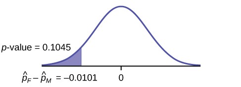
Researchers conducted a study of smartphone use among adults. A cell phone company claimed that iPhone smartphones are more popular with whites (non-Hispanic) than with African Americans. The results of the survey indicate that of the 232 African American cell phone owners randomly sampled, 5% have an iPhone. Of the 1,343 white cell phone owners randomly sampled, 10% own an iPhone. Test at the 5% level of significance. Is the proportion of white iPhone owners greater than the proportion of African American iPhone owners?
- Step 1: Define the hypotheses
- (H_0: p_W = p_A) (The proportion of white iPhone owners is equal to the proportion of African American iPhone owners.)
- (H_1: p_W > p_A) (The proportion of white iPhone owners is greater than the proportion of African American iPhone owners.)
- Step 2: Calculate the pooled proportion
[p_c = frac{(0.10 1343) + (0.05 232)}{1343 + 232} = 0.0927] - Step 3: Calculate the test statistic
[z = frac{0.10 – 0.05}{sqrt{0.0927(1 – 0.0927)left(frac{1}{1343} + frac{1}{232}right)}} = 2.33] - Step 4: Determine the p-value
- Since this is a right-tailed test, the p-value is (P(Z > 2.33) = 0.0099).
- Step 5: Make a decision
- Since the p-value (0.0099) is less than the significance level (0.05), we reject the null hypothesis.
- Step 6: State the conclusion
- At the 5% level of significance, there is sufficient evidence to conclude that a larger proportion of white cell phone owners use iPhones than African Americans.
7.3. Example 3: Dog Adoption Rates
How much more likely are puppies in the animal shelter to be adopted in their first week there compared to older dogs? 278 of the 321 puppies sampled were adopted in the first week and 472 of the 649 older dogs were adopted in the first week.
- Step 1: Define the sample proportions
- Puppies: (hat{p}_1 = frac{278}{321} approx 0.866)
- Older Dogs: (hat{p}_2 = frac{472}{649} approx 0.727)
- Step 2: Calculate the confidence interval
- Using the formula for a 95% confidence interval, we find the interval to be approximately [0.0828, 0.1948].
- Step 3: State the conclusion
- With 95% confidence, puppies are between 8% and 19% more likely than older dogs to be adopted in their first week at the shelter.
8. Common Pitfalls to Avoid
When conducting a two-proportion test, it’s important to be aware of common pitfalls that can lead to incorrect conclusions.
8.1. Violating Assumptions
One of the most common pitfalls is violating the assumptions of the test. If the assumptions of independence, random sampling, and sample size are not met, the test results may be unreliable.
8.2. Misinterpreting P-values
The p-value is often misinterpreted as the probability that the null hypothesis is true. However, the p-value is the probability of observing the data, or data more extreme, assuming the null hypothesis is true. It does not tell us the probability that the null hypothesis is true.
8.3. Confusing Statistical Significance with Practical Significance
A statistically significant result does not necessarily mean that the result is practically significant. A small difference in proportions may be statistically significant if the sample sizes are large, but the difference may not be meaningful in practice.
8.4. Data Dredging
Data dredging, also known as p-hacking, is the practice of repeatedly testing different hypotheses until a statistically significant result is found. This can lead to false positives and should be avoided.
9. Tools and Resources
Several tools and resources can assist in conducting a two-proportion test.
9.1. Statistical Software
Statistical software packages such as R, Python, SPSS, and SAS can be used to perform two-proportion tests and calculate confidence intervals. These software packages provide a wide range of statistical functions and can handle large datasets.
9.2. Online Calculators
Several online calculators can be used to perform two-proportion tests. These calculators are easy to use and do not require any programming or statistical knowledge.
9.3. Textbooks and Articles
Numerous textbooks and articles provide detailed explanations of the two-proportion test and its applications. These resources can be helpful for understanding the theoretical foundations of the test and its assumptions.
10. The Importance of Context
Statistical tests are powerful tools, but they should always be interpreted in the context of the problem being studied. Consider the following:
10.1. Practical Significance
Even if a difference is statistically significant, it may not be practically significant. For example, a new drug might reduce the risk of a disease by a statistically significant amount, but if the reduction is only 0.1%, it may not be worth the cost and potential side effects.
10.2. Confounding Variables
A statistically significant difference between two proportions may be due to a confounding variable, rather than a causal relationship. For example, a study might find that people who drink coffee are more likely to develop a certain disease. However, this could be because coffee drinkers are also more likely to smoke, and smoking is the actual cause of the disease.
10.3. Bias
Bias can affect the results of any statistical test. It is important to be aware of potential sources of bias and to take steps to minimize their impact.
11. Advanced Topics
For those who want to delve deeper into the topic, here are some advanced topics related to comparing two proportions.
11.1. Power Analysis
Power analysis is used to determine the sample size needed to detect a statistically significant difference between two proportions. A power analysis can help ensure that the study has enough power to detect a meaningful difference.
11.2. Non-parametric Tests
Non-parametric tests can be used to compare two proportions when the assumptions of the two-proportion test are not met. These tests do not rely on the assumption that the data are normally distributed.
11.3. Bayesian Methods
Bayesian methods provide an alternative approach to hypothesis testing. Bayesian methods allow us to calculate the probability that the null hypothesis is true, given the data.
12. COMPARE.EDU.VN: Your Partner in Statistical Analysis
At COMPARE.EDU.VN, we understand the challenges of statistical analysis and decision-making. That’s why we’re committed to providing you with the tools and resources you need to succeed. Whether you’re comparing products, services, or ideas, we’re here to help you make informed decisions.
12.1. Comprehensive Comparisons
We offer comprehensive comparisons across a wide range of topics. Our in-depth analysis covers all the key factors you need to consider, including features, pros and cons, and user reviews.
12.2. Unbiased Information
We are committed to providing unbiased information. Our comparisons are based on objective data and thorough research, ensuring that you get the most accurate and reliable information possible.
12.3. User-Friendly Interface
Our website is designed to be user-friendly. You can easily find the comparisons you’re looking for and quickly see the key differences between your options.
13. Frequently Asked Questions (FAQs)
To further clarify the concepts and procedures discussed in this guide, here are some frequently asked questions about comparing two proportions using a statistical test.
13.1. What does it mean to compare two proportions?
Comparing two proportions means assessing whether the difference between the proportions of two independent groups is statistically significant or due to random chance. It is a statistical method used to determine if two population proportions are different.
13.2. What are the assumptions required for the two-proportion test?
The assumptions include:
- The two samples are independent.
- Both samples are randomly selected.
- Sample sizes are sufficiently large (np ≥ 5 and n(1-p) ≥ 5 for both samples).
- The populations are at least ten times the size of the samples.
13.3. How do I choose the right alternative hypothesis?
Choose the alternative hypothesis based on the research question:
- Two-tailed ((H_1: p_1 neq p_2)): Use when you want to test if there is any difference between the proportions.
- Left-tailed ((H_1: p_1 < p_2)): Use when you want to test if the proportion of the first group is less than the proportion of the second group.
- Right-tailed ((H_1: p_1 > p_2)): Use when you want to test if the proportion of the first group is greater than the proportion of the second group.
13.4. What is the significance level, and how is it chosen?
The significance level ((alpha)) is the probability of rejecting the null hypothesis when it is true (Type I error). It is typically set at 0.05, meaning there is a 5% chance of rejecting the null hypothesis when it is true.
13.5. How is the pooled proportion calculated?
The pooled proportion (p_c) is calculated as:
[p_c = frac{x_1 + x_2}{n_1 + n_2}]
Where (x_1) and (x_2) are the number of successes in the first and second samples, and (n_1) and (n_2) are the sample sizes of the first and second samples.
13.6. What does the p-value tell us?
The p-value indicates the probability of observing a test statistic as extreme as, or more extreme than, the one calculated, assuming the null hypothesis is true.
13.7. How do I interpret the p-value in the context of a hypothesis test?
- If (ptext{-value} leq alpha), reject the null hypothesis.
- If (ptext{-value} > alpha), fail to reject the null hypothesis.
13.8. What is a confidence interval for the difference between two proportions, and how do I interpret it?
A confidence interval provides a range of plausible values for the true difference between two population proportions. For example, a 95% confidence interval means we are 95% confident that the true difference lies within the calculated interval.
13.9. What are common pitfalls to avoid when conducting a two-proportion test?
Common pitfalls include violating assumptions, misinterpreting p-values, confusing statistical significance with practical significance, and data dredging.
13.10. Where can I find tools and resources to help me conduct a two-proportion test?
Tools and resources include statistical software (e.g., R, Python, SPSS), online calculators, and textbooks or articles on statistical methods.
14. Conclusion: Empowering Your Decision-Making
The “How To Compare Two Proportions Statistical Test” is an essential tool for anyone looking to make data-driven decisions. By understanding the underlying principles, following the steps outlined in this guide, and avoiding common pitfalls, you can confidently analyze data and draw meaningful conclusions. Remember to always consider the context of your analysis and to interpret your results with caution.
At COMPARE.EDU.VN, we are dedicated to providing you with the resources you need to make informed decisions. We invite you to explore our website and discover the many ways we can help you compare your options and make the best choice for your needs. Whether you’re a student, a consumer, or a professional, we’re here to support you every step of the way.
Ready to start comparing? Visit COMPARE.EDU.VN today and unlock the power of informed decision-making.
Contact us:
Address: 333 Comparison Plaza, Choice City, CA 90210, United States
Whatsapp: +1 (626) 555-9090
Website: COMPARE.EDU.VN
Navigate the complexities of statistical comparisons with ease and precision at compare.edu.vn, ensuring every choice is backed by thorough analysis and informed insights.