Comparing two numbers in Excel is a fundamental skill for data analysis, financial modeling, and various other tasks. Are you struggling to compare two numbers or columns in Excel? COMPARE.EDU.VN provides an efficient and comprehensive guide on how to compare numbers in Excel and streamline your data analysis. Learn the best methods for number comparison, including built-in functions and conditional formatting, to unlock hidden patterns in your data.
Are you looking for a more efficient way to compare data, spot discrepancies, and make data-driven decisions using Excel? Explore advanced techniques, such as the EXACT function and lookup formulas, to enhance your analytical capabilities. Visit COMPARE.EDU.VN today for more insights on data comparison techniques and data analysis.
1. Why Comparing Numbers Is Useful In Excel
Excel is a powerful tool for data storage, analysis, and decision-making. Comparing numbers is crucial for identifying trends, discrepancies, and patterns that can inform critical business decisions. Data analysts rely on number comparisons to gather insights that drive marketing and sales strategies.
When working with large datasets or linked spreadsheets, even a single incorrect cell can have significant consequences. The impact of missing or inaccurate information highlights the importance of data analysts being able to compare columns and identify any discrepancies quickly and accurately. Manually comparing columns is time-consuming and prone to error. Automating this process can save hours of work and ensure data integrity.
Comparing two columns in Excel allows data analysts to quickly identify whether a cell contains data or not. Excel can display results as TRUE/FALSE, Match/Not Match, or custom messages, making it easy to spot differences.
2. Essential Methods To Compare Two Numbers In Excel
When you have data in different columns, tables, or spreadsheets, comparing them becomes essential to identify missing or duplicate entries. Depending on your goals, various comparison methods are available in Excel. The right method will depend on what you want to achieve from the comparison. You can compare two columns in Excel using the following techniques:
- Highlight unique or duplicate values using functions.
- Display unique or duplicate values using conditional formatting or formulas.
- Perform row-by-row comparisons.
- Utilize LOOKUP formulas.
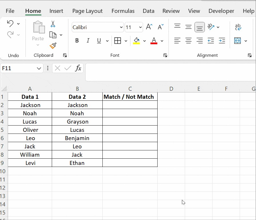
3. Comparing Two Numbers Using The Equals Operator
You can compare two columns row by row to find matching data, displaying the result as “Match” or “Not Match.” For example, the formula =A2=B2 identifies matching data, returning TRUE if the values in the compared rows are identical and FALSE otherwise.
To use this method, enter the formula in cell C2 and drag it down to the end of the table. This will quickly show which rows have the same values and which do not.
3.1. Using the IF Condition to Compare Numbers
In Excel, the IF condition provides a way to compare two columns. The formula =IF(A2=B2,”Match”,” “) returns “Match” for rows with identical values and leaves the remaining rows empty.
This formula can be modified to identify mismatching values by providing an alternative result when the IF condition is false. For example, =IF(A2=B2,”Match”,”Not a Match”) displays “Match” for matching values and “Not a Match” for different values.
To compare columns for differences, use the non-equality sign (<>) instead of the equals sign (=). The formula =IF(A2<>B2,”Match”,”Not a Match”) returns “Match” for different values and “Not a Match” for matching values.
3.2. Using the EXACT() Function For Case-Sensitive Number Comparisons
The EXACT() function is useful when you need to compare two columns in a case-sensitive manner. It compares two text strings and returns TRUE if they are identical, including case, and FALSE otherwise. Formatting differences are ignored. The syntax is =EXACT(text1, text2), where both text1 and text2 are required arguments.
Consider an example where columns A and B contain the text strings “Nova Scotia”.
Applying the formula =IF(A2=B2, “Match”, “Mismatch”) to cell C2 returns “Match” because the comparison is case-insensitive.
However, using the formula =IF(EXACT(A2, B2), “Match”, “Mismatch”) makes the comparison case-sensitive.
The EXACT() function returns TRUE or FALSE. The IF condition evaluates this result and returns the appropriate message. If EXACT() returns TRUE, the IF condition returns “Match”; otherwise, it returns “Mismatch”.
4. Conditional Formatting For Number Comparisons
Conditional formatting is a powerful tool for highlighting unique or duplicate numbers in Excel. To use this feature, follow these steps:
- Click Home in the Excel ribbon.
- Go to the Styles group.
- Select Conditional Formatting.
- Choose Highlight Cell Rules.
- Click Duplicate Values.
A dialogue box will appear, allowing you to customize the formatting. You can choose to highlight Duplicate or Unique values and select a formatting style from the options provided.
4.1. Highlighting Duplicate Numbers
Highlighting duplicate numbers is useful when you want to identify values that appear in both columns. Select both columns of data and follow the steps mentioned above. Choose Duplicate from the drop-down menu. Then, select a formatting option like filling with color, changing the text color, or altering the cell border.
For more customization, choose Custom Format to select a color of your choice.
4.2. Highlighting Unique Numbers
Highlighting unique numbers is useful when you want to identify values that appear only in one column. Select both columns of data, go to Conditional Formatting, and choose Unique from the drop-down list. Apply a formatting option such as filling with color, changing the text color, or changing the cell border.
4.3. Clearing Conditional Formatting Rules
To clear the formatting rules you’ve applied, click Conditional Formatting → Clear Rules → Clear Rules from Selected Cells.
Conditional formatting is ideal when you want to highlight matching or different numbers without adding a third column. However, for larger spreadsheets, more complex methods may be required.
5. Using Lookup Functions to Compare Two Columns
Lookup functions search for a value in a row or column and return a corresponding value from another row or column. Excel offers several lookup functions, including HLOOKUP, VLOOKUP, and XLOOKUP. VLOOKUP is particularly useful for comparing columns and identifying matching or missing data.
5.1. Using VLOOKUP to Compare Numbers
VLOOKUP can compare two columns to identify differences. For example, column A might contain a list of exams taken by a student, and column B might list the subjects the student passed. To find which subjects the student has not passed, you can use VLOOKUP.
Apply the formula =VLOOKUP(A2, $B$2:$B$5,1,0) in cell C2 and drag it down to apply it to all cells below C2. Column C will show the subjects that have been cleared and those that have not been cleared, indicated by #N/A.
Understanding the VLOOKUP Formula:
- VLOOKUP(A2,..,..,..) – takes the value in cell A2.
- VLOOKUP(A2, $B$2:$B$5,..,..) – compares with all the values in cells from B2 to B5. The $ symbol before the cell reference is called an absolute reference, locking the cells in the range B2:B5.
- VLOOKUP(A2, $B$2:$B$5,1,..) – the third argument is the col_index_num, which specifies the position of the column to compare from the lookup value A2. In this example, the subjects list is in column A, and the column to compare with is one column away. Hence, the value is 1.
- VLOOKUP(A2, $B$2:$B$5,1,0) – the last argument takes a logical value, either 0 or 1. Use 0 to find an exact match and 1 to find the closest match sorted in ascending order.
6. Comparing Numbers In Excel: FAQ
6.1. How do I compare two columns in Excel to find differences?
To compare two columns in Excel to find differences, select both columns of data, select Home → Find & Select → Go To Special → Row Differences, and click OK. The matching data cells across the columns’ rows are white, and unmatched cells appear in gray.
6.2. What are other methods to compare two columns in Excel using the IF condition?
To find matches in all cells within the same row when the table has three or more columns, use an IF formula with an AND statement. The formula is =IF(AND(A2=B2, A2=C2), “Full match”, “”).
To find matches in any two cells in the same row, use the formula =IF(OR(A2=B2, B2=C2, A2=C2), “Match”, “”).
6.3. Can you compare two columns in Excel using the Index-Match function?
Yes, you can use the INDEX-MATCH function to compare two columns and pull matching entries from another table. The MATCH() function compares values in one column with those in another column. If it finds a match, it pulls the corresponding value from another column; otherwise, it returns #N/A.
7. Conclusion
Comparing numbers in Excel is an essential skill for data analysis and decision-making. Microsoft Excel provides various methods to compare and match numbers in single or multiple columns and spreadsheets. This guide has shown you several methods to compare two columns for matches.
Lookup functions are vital to learn in Excel due to their wide usage. Visit COMPARE.EDU.VN for more in-depth tutorials and courses on Excel functions and formulas, as well as micro-credentials upon completion. For further assistance, contact us at 333 Comparison Plaza, Choice City, CA 90210, United States, or via WhatsApp at +1 (626) 555-9090. Enhance your data analysis skills and make informed decisions with compare.edu.vn.