How to Compare Two Months Data in Excel

Comparing two months of data in Excel provides crucial insights for informed decision-making. compare.edu.vn offers solutions to streamline this process, empowering users to effectively analyze and compare data sets. Discover techniques to enhance your data analysis skills.

1. Understanding the Basics of Data Comparison in Excel

Before diving into specific methods, it’s essential to grasp the fundamental principles of data comparison in Excel. This involves understanding how to organize your data, utilize basic formulas, and leverage Excel’s built-in functions for comparing data sets. Data comparison is the process of identifying similarities and differences between two or more sets of data. This involves examining data points for variations in value, type, structure, or format. In Excel, data comparison often entails comparing values in different cells, rows, or columns to identify trends, anomalies, or patterns.

1.1. Organizing Data for Comparison

The first step in any data comparison task is to ensure that your data is organized in a structured and consistent manner. This typically involves arranging your data into tables or spreadsheets, with each column representing a specific variable or attribute and each row representing a data point or observation. By organizing your data in this way, you can easily compare values across different rows or columns and identify meaningful insights.

For example, if you’re comparing sales data for two different months, you might organize your data into a table with columns for date, product, quantity sold, and revenue. Each row would represent a single transaction or sale, and you could then compare the values in each column across the two months to identify changes in sales performance.

1.2. Utilizing Basic Formulas for Comparison

Excel offers a variety of built-in formulas that can be used to compare data sets and identify differences or similarities. These formulas can be used to perform simple comparisons, such as checking if two values are equal, or more complex comparisons, such as calculating the percentage change between two values.

Some of the most commonly used formulas for data comparison include:

=IF(A1=B1, "Match", "No Match"): This formula compares the values in cells A1 and B1 and returns “Match” if they are equal and “No Match” if they are not equal.
=A1-B1: This formula calculates the difference between the values in cells A1 and B1.
=(A1-B1)/B1: This formula calculates the percentage change between the values in cells A1 and B1.

By utilizing these basic formulas, you can quickly and easily compare data sets in Excel and identify meaningful insights.

1.3. Leveraging Excel’s Built-In Functions for Comparison

In addition to basic formulas, Excel also offers a variety of built-in functions that can be used to compare data sets and perform more complex analyses. These functions can be used to identify duplicate values, find the maximum or minimum value in a range of cells, or perform statistical analyses on your data.

Some of the most commonly used functions for data comparison include:

COUNTIF(range, criteria): This function counts the number of cells in a range that meet a specific criteria.
SUMIF(range, criteria, sum_range): This function sums the values in a range that meet a specific criteria.
AVERAGEIF(range, criteria, average_range): This function calculates the average of the values in a range that meet a specific criteria.
VLOOKUP(lookup_value, table_array, col_index_num, [range_lookup]): This function searches for a value in the first column of a table and returns the value in the same row from a specified column.

By leveraging these built-in functions, you can perform more sophisticated data comparisons in Excel and gain deeper insights into your data.

2. Comparing Data Using Formulas and Functions

Excel provides a wide array of formulas and functions that facilitate data comparison. We will explore some of the most commonly used methods, including the IF function, comparison operators, and specialized functions for specific comparison tasks. Formulas and functions are essential tools for performing data comparison in Excel, offering flexibility and precision in analyzing datasets. These tools enable users to identify similarities, differences, trends, and patterns within their data, empowering them to make informed decisions.

2.1. Using the IF Function for Basic Comparisons

The IF function is a fundamental tool for performing basic comparisons in Excel. It allows you to test a condition and return one value if the condition is true and another value if the condition is false. The syntax of the IF function is as follows:

=IF(logical_test, value_if_true, value_if_false)

Where:

logical_test is the condition that you want to test.
value_if_true is the value that you want to return if the condition is true.
value_if_false is the value that you want to return if the condition is false.

For example, if you want to compare the sales figures for two months and determine whether sales increased or decreased, you can use the IF function as follows:

=IF(B2>A2, "Increase", "Decrease")

Where:

A2 contains the sales figures for the first month.
B2 contains the sales figures for the second month.

This formula will return “Increase” if the sales figures for the second month are greater than the sales figures for the first month, and “Decrease” otherwise.

2.2. Utilizing Comparison Operators for Equality and Inequality Checks

Comparison operators are used to compare two values and determine their relationship. Excel provides a variety of comparison operators, including:

=: Equal to
>: Greater than
<: Less than
>=: Greater than or equal to
<=: Less than or equal to
<>: Not equal to

These operators can be used in conjunction with the IF function or other formulas to perform more complex comparisons. For example, if you want to check whether the sales figures for two months are equal, you can use the following formula:

=IF(A2=B2, "Equal", "Not Equal")

This formula will return “Equal” if the sales figures for the two months are equal and “Not Equal” otherwise.

2.3. Employing Specialized Functions for Specific Comparison Tasks

In addition to the IF function and comparison operators, Excel also provides a variety of specialized functions that can be used for specific comparison tasks. These functions include:

EXACT(text1, text2): This function compares two text strings and returns TRUE if they are exactly the same and FALSE otherwise.
DELTA(number1, number2): This function compares two numbers and returns 1 if they are equal and 0 otherwise.
SIGN(number): This function returns the sign of a number (-1 for negative, 0 for zero, and 1 for positive).

These functions can be particularly useful for comparing text strings, identifying duplicate values, or analyzing trends in your data.

Show The Difference From Previous Months With Excel Pivot Tables

3. Leveraging Conditional Formatting for Visual Data Comparison

Conditional formatting allows you to visually highlight data based on specific criteria. This technique can be incredibly useful for quickly identifying trends, outliers, and significant changes in your data. Conditional formatting is a powerful feature in Excel that enables users to visually highlight cells or ranges of cells based on specific criteria. This allows for quick identification of patterns, trends, outliers, and significant changes within a dataset, making it an invaluable tool for data analysis and comparison.

3.1. Highlighting Differences with Color Scales

Color scales are a type of conditional formatting that allows you to apply a gradient of colors to a range of cells based on their values. This can be particularly useful for highlighting differences in data over time.

For example, if you want to compare the sales figures for two months and highlight the products that experienced the largest increase or decrease in sales, you can use a color scale to apply a gradient of colors to the sales figures, with the highest values being colored green and the lowest values being colored red.

To apply a color scale to a range of cells, follow these steps:

Select the range of cells that you want to format.
Click on the “Conditional Formatting” button in the “Home” tab.
Select “Color Scales” from the drop-down menu.
Choose the color scale that you want to apply.

Excel will automatically apply the color scale to the selected range of cells, highlighting the differences in the data.

3.2. Using Icon Sets to Indicate Trends

Icon sets are another type of conditional formatting that allows you to display icons in cells based on their values. This can be particularly useful for indicating trends in data over time.

For example, if you want to compare the sales figures for two months and indicate whether sales increased, decreased, or remained the same, you can use an icon set to display an up arrow for increased sales, a down arrow for decreased sales, and a horizontal arrow for unchanged sales.

To apply an icon set to a range of cells, follow these steps:

Select the range of cells that you want to format.
Click on the “Conditional Formatting” button in the “Home” tab.
Select “Icon Sets” from the drop-down menu.
Choose the icon set that you want to apply.

Excel will automatically apply the icon set to the selected range of cells, indicating the trends in the data.

3.3. Creating Custom Rules for Advanced Highlighting

In addition to the built-in conditional formatting options, Excel also allows you to create custom rules for advanced highlighting. This can be particularly useful for highlighting data based on specific criteria or conditions.

For example, if you want to highlight the products that experienced a sales increase of more than 10% or a sales decrease of more than 10%, you can create a custom rule that applies a specific format to the cells that meet these criteria.

To create a custom rule for conditional formatting, follow these steps:

Select the range of cells that you want to format.
Click on the “Conditional Formatting” button in the “Home” tab.
Select “New Rule” from the drop-down menu.
Choose the rule type that you want to create.
Enter the criteria or conditions for the rule.
Choose the format that you want to apply.

Excel will automatically apply the custom rule to the selected range of cells, highlighting the data that meets the specified criteria.

4. Utilizing Pivot Tables for Month-to-Month Data Analysis

Pivot tables offer a powerful way to summarize and analyze large datasets. This section will guide you through creating pivot tables to compare month-to-month data, calculate differences, and display results in a meaningful way. Pivot tables are a powerful feature in Excel that allows users to summarize, analyze, and visualize large datasets with ease. They provide a flexible and interactive way to explore data from different perspectives, identify trends, and extract meaningful insights.

4.1. Creating a Pivot Table for Month-to-Month Comparison

To create a pivot table for month-to-month comparison, follow these steps:

Select the data range that you want to analyze.
Click on the “Insert” tab in the Excel ribbon.
Click on the “PivotTable” button.
In the “Create PivotTable” dialog box, choose the data range and the location where you want to place the pivot table.
Click “OK” to create the pivot table.

Once the pivot table is created, you can drag and drop the fields that you want to analyze into the different areas of the pivot table. For month-to-month comparison, you will typically drag the “Date” field into the “Rows” area, the “Sales” field into the “Values” area, and the “Month” field into the “Columns” area.

Excel will automatically group the data by month and calculate the sum of sales for each month. You can then use the pivot table’s filtering and sorting capabilities to further analyze the data and identify trends.

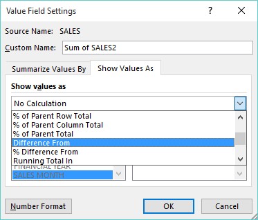
4.2. Calculating Differences between Months in a Pivot Table

To calculate the differences between months in a pivot table, follow these steps:

Right-click on the “Sales” field in the “Values” area of the pivot table.
Select “Show Values As” from the context menu.
Choose “Difference From” from the list of options.
In the “Base field” drop-down menu, select “Month”.
In the “Base item” drop-down menu, select “(previous)”.
Click “OK” to calculate the differences between months.

Excel will automatically calculate the difference between the sales figures for each month and display the results in the pivot table. You can then use conditional formatting or other techniques to highlight the significant changes in sales over time.

4.3. Displaying Results in a Meaningful Way

To display the results of your month-to-month data analysis in a meaningful way, you can use a variety of techniques, such as:

Creating charts and graphs: Excel provides a variety of chart and graph types that can be used to visualize the data in your pivot table. This can help you to quickly identify trends and patterns in the data.
Using conditional formatting: Conditional formatting can be used to highlight the significant changes in sales over time. This can help you to quickly identify the months that experienced the largest increase or decrease in sales.
Adding calculated fields: Calculated fields can be used to perform additional calculations on the data in your pivot table. For example, you can add a calculated field to calculate the percentage change in sales from one month to the next.
Using slicers and filters: Slicers and filters can be used to narrow down the data that is displayed in your pivot table. This can help you to focus on the specific areas of the data that you are most interested in.

By using these techniques, you can effectively display the results of your month-to-month data analysis and communicate your findings to others.

5. Visual Aids: Enhancing Your Month-to-Month Data

Visual aids play a crucial role in the comprehension of data, more so when you want to depict changes over time, like month-to-month fluctuations. Visual aids are powerful tools for enhancing the comprehension of data, particularly when depicting changes over time, such as month-to-month fluctuations. By incorporating visual elements into data presentations, analysts can effectively communicate complex information, highlight trends, and facilitate decision-making.

5.1. Directional Icons for Quick Insights

By incorporating directional icons into your spreadsheets, you equip yourself and your audience with the ability to capture the essence of the data at a glance. Imagine icons that rise or dip, offering immediate insight into trends without poring over each number—this is the convenience directional icons offer. They represent increases, decreases, and steadiness with upward arrows, downward arrows, and dashes, respectively.

To insert directional icons into your Excel spreadsheet, follow these steps:

Select the cells that you want to format with directional icons.
Click on the “Conditional Formatting” button in the “Home” tab.
Select “Icon Sets” from the drop-down menu.
Choose the directional icon set that you want to apply.

Excel will automatically apply the directional icons to the selected cells, indicating the trends in the data.

5.2. Conditional Formatting for Clarity and Impact

Conditional formatting can dramatically increase the clarity and impact of your data visualization. With Excel’s rich set of formatting rules, you can highlight month-to-month changes in a way that brings immediate attention to important trends. For example, you might use a gradient color scale to show varying degrees of increase or decrease, or apply a specific color to represent significant shifts.

To set this up, simply select the % change column in your spreadsheet, navigate to “Home > Conditional Formatting > New Rule,” and specify your rule to reflect the desired visual effect.

Conditional formatting offers a wide range of options for visually highlighting data based on specific criteria. You can use color scales to represent the magnitude of values, icon sets to indicate trends, or data bars to compare values side-by-side. By experimenting with different conditional formatting options, you can create visualizations that effectively communicate the insights hidden within your data.

6. Advanced Tips for Excel Data Analysis

As you become more proficient with comparing data in Excel, you can explore advanced techniques for even more insightful analysis. As users become more proficient in comparing data in Excel, they can explore advanced techniques to unlock even more profound insights and streamline their analysis processes. These advanced tips encompass a range of strategies, from leveraging pivot table value settings to handling common errors and issues, ultimately empowering users to extract maximum value from their data.

6.1. Dealing with Common Errors and Issues

Working with spreadsheets to show month-to-month changes often leads to encounters with errors or unexpected results, especially when using ‘Difference From’ or ‘% Difference From’ settings. Errors might manifest as baffling messages, or you could observe issues when attempting changes. To navigate around these bumps, an understanding of why these errors arise is invaluable.

A common error may be a result of data fields moving or becoming renamed, leading to invalid references. Always double-check your data sources and field names. Another hiccup occurs when calculations on blank cells or zeroes return errors or divide-by-zero results. In this case, ensure you have complete data or consider using custom formulas that account for these possibilities.

To mitigate these errors, users can implement error-handling techniques such as using the IFERROR function to handle division-by-zero errors or employing data validation rules to ensure data integrity. Additionally, regularly reviewing data sources and field names can prevent invalid references and ensure accurate calculations.

6.2. Leveraging More Excel Value Settings

Diving deeper into spreadsheet value settings opens up a universe of data analysis possibilities. You’re not just limited to displaying sums or counts; you can customize your spreadsheet to perform a variety of calculations, such as averages, maximums, minimums, or more sophisticated computations like running totals or percentiles.

To access these, right-click on a value within your spreadsheet and explore the ‘Summarize Values By’ and ‘Show Values As’ options. For month-to-month analysis, you might select ‘Difference From’ to view the absolute change or ‘% Difference From’ for the relative change from one month to the next. Each selection dynamically reshapes your data’s story, giving you the analytical edge.

By leveraging Excel’s value settings, users can gain deeper insights into their data, uncover hidden patterns, and make more informed decisions. Experimenting with different value settings can reveal new perspectives and enhance the overall effectiveness of data analysis in Excel.

6.3. Utilizing Sparklines for Inline Data Visualization

Sparklines are small, inline charts that fit within a single cell and provide a visual representation of data trends. They are particularly useful for visualizing month-to-month changes in data, as they allow you to quickly see the overall trend without taking up much space.

To insert sparklines into your Excel spreadsheet, follow these steps:

Select the cells where you want to insert the sparklines.
Click on the “Insert” tab in the Excel ribbon.
In the “Sparklines” group, choose the type of sparkline that you want to insert (e.g., line, column, or win/loss).
In the “Data Range” box, select the range of cells that contains the data that you want to visualize.
Click “OK” to insert the sparklines.

Excel will automatically insert the sparklines into the selected cells, providing a visual representation of the data trends.

7. Best Practices for Excel Data Comparison

To ensure accurate and reliable data comparisons, it’s essential to follow best practices for data entry, data validation, and documentation. To ensure accurate, reliable, and meaningful data comparisons in Excel, it’s imperative to adhere to a set of best practices encompassing data entry, validation, documentation, and security measures. These practices not only enhance the integrity of the data but also streamline the analysis process, enabling users to derive valuable insights with confidence.

7.1. Ensuring Data Accuracy and Consistency

Data accuracy and consistency are paramount for reliable data comparisons. Implement data validation rules to ensure that data is entered correctly and consistently. This can help to prevent errors and ensure that your comparisons are based on accurate data.

Data validation rules can be used to restrict the type of data that can be entered into a cell, such as numbers, dates, or text. They can also be used to specify a range of values that are allowed, or to create a drop-down list of valid options.

By implementing data validation rules, you can significantly reduce the risk of data entry errors and ensure that your comparisons are based on accurate and consistent data.

7.2. Documenting Your Comparison Process

Documenting your comparison process is essential for reproducibility and transparency. Keep a record of the steps that you took to compare the data, the formulas and functions that you used, and any assumptions that you made.

This documentation will help you to reproduce the comparison at a later date, and it will also help others to understand your analysis and to verify your results.

7.3. Securing Your Data and Protecting Your Analysis

Data security is crucial for protecting your sensitive information. Implement security measures to protect your data from unauthorized access and modification. This can include password protecting your spreadsheet, encrypting sensitive data, and restricting access to the spreadsheet.

By implementing these security measures, you can ensure that your data is protected from unauthorized access and that your analysis remains confidential.

8. Automating Data Comparison with Macros

For repetitive data comparison tasks, consider using macros to automate the process. Macros can save you time and effort by automating the steps involved in comparing data. For repetitive data comparison tasks, leveraging macros offers a streamlined approach to automate the entire process. Macros, essentially snippets of code written in Visual Basic for Applications (VBA), enable users to automate a series of actions within Excel, saving time, reducing manual errors, and enhancing overall efficiency.

8.1. Recording a Macro for Simple Comparisons

To record a macro for simple comparisons, follow these steps:

Click on the “View” tab in the Excel ribbon.
Click on the “Macros” button.
Select “Record Macro” from the drop-down menu.
In the “Record Macro” dialog box, enter a name for the macro and a description.
Click “OK” to start recording the macro.
Perform the steps that you want to automate.
Click on the “Stop Recording” button in the Excel ribbon to stop recording the macro.

Excel will automatically generate the VBA code for the macro. You can then run the macro to automate the steps that you recorded.

8.2. Editing the Macro for Customization

To edit the macro for customization, follow these steps:

Click on the “View” tab in the Excel ribbon.
Click on the “Macros” button.
Select “View Macros” from the drop-down menu.
In the “Macros” dialog box, select the macro that you want to edit.
Click “Edit” to open the VBA editor.
Modify the VBA code as needed.
Click “Save” to save the changes.

You can use the VBA editor to customize the macro to perform more complex comparisons or to automate additional tasks.

8.3. Assigning the Macro to a Button or Shortcut

To assign the macro to a button or shortcut, follow these steps:

Click on the “Developer” tab in the Excel ribbon.
Click on the “Insert” button in the “Controls” group.
Choose the type of control that you want to insert (e.g., button, checkbox, or option button).
Draw the control on the spreadsheet.
Right-click on the control and select “Assign Macro” from the context menu.
In the “Assign Macro” dialog box, select the macro that you want to assign to the control.
Click “OK” to assign the macro to the control.

You can also assign a shortcut key to the macro by editing the macro in the VBA editor and adding a Sub statement with the ShortcutKey property.

9. Troubleshooting Common Data Comparison Issues

Even with careful planning and execution, data comparison tasks can sometimes encounter issues. This section will address some common problems and provide solutions for resolving them. Even with meticulous planning and execution, data comparison tasks may encounter various issues that impede the accuracy and efficiency of the analysis. Addressing these common problems requires a systematic approach involving troubleshooting techniques, error handling strategies, and data validation methods.

9.1. Handling Mismatched Data Types

One common issue is mismatched data types. Ensure that the data you are comparing is of the same type (e.g., numbers, text, dates). If the data types are different, you may need to convert them to a common type before comparing them.

Excel provides a variety of functions for converting data types, such as VALUE, TEXT, and DATE. You can use these functions to convert the data to a common type before comparing them.

9.2. Dealing with Inconsistent Formatting

Inconsistent formatting can also cause problems with data comparison. Ensure that the data is formatted consistently (e.g., number of decimal places, date format). If the formatting is inconsistent, you may need to reformat the data before comparing it.

Excel provides a variety of formatting options that you can use to format the data consistently. You can use the “Format Cells” dialog box to specify the number of decimal places, date format, and other formatting options.

9.3. Resolving Errors in Formulas and Functions

Errors in formulas and functions can also cause problems with data comparison. Double-check your formulas and functions to ensure that they are correct and that they are referencing the correct cells.

Excel provides a variety of tools for debugging formulas and functions, such as the “Evaluate Formula” tool and the “Error Checking” tool. You can use these tools to identify and resolve errors in your formulas and functions.

10. Advanced Data Analysis Techniques in Excel

For users seeking to go beyond basic data comparison, Excel offers advanced techniques such as statistical analysis and data mining. For users aspiring to transcend basic data comparison and delve into more sophisticated insights, Excel offers a repertoire of advanced techniques, including statistical analysis, data mining, and predictive modeling. These advanced capabilities empower users to uncover hidden patterns, trends, and relationships within their data, facilitating more informed decision-making and strategic planning.

10.1. Performing Statistical Analysis for Deeper Insights

Excel provides a variety of statistical functions that you can use to perform statistical analysis on your data. These functions can help you to identify trends, patterns, and relationships in your data.

Some of the most commonly used statistical functions include:

AVERAGE: Calculates the average of a range of numbers.
MEDIAN: Calculates the median of a range of numbers.
STDEV: Calculates the standard deviation of a range of numbers.
CORREL: Calculates the correlation between two ranges of numbers.
T.TEST: Performs a t-test to compare the means of two groups.

10.2. Utilizing Data Mining Tools for Pattern Discovery

Excel also provides a variety of data mining tools that you can use to discover patterns in your data. These tools can help you to identify clusters of similar data points, to predict future values based on past data, and to identify outliers in your data.

Some of the most commonly used data mining tools include:

Cluster Analysis: Groups similar data points together.
Regression Analysis: Predicts future values based on past data.
Outlier Analysis: Identifies outliers in your data.

10.3. Creating Predictive Models for Future Trends

Excel also allows you to create predictive models to forecast future trends based on your historical data. This can be particularly useful for forecasting sales, demand, or other key business metrics.

You can use a variety of techniques to create predictive models in Excel, such as regression analysis, time series analysis, and exponential smoothing.

FAQ: Excel Data Comparison – Your Questions Answered

Here are some frequently asked questions about comparing data in Excel:

1. How do I compare two columns in Excel for differences?

To compare two columns in Excel for differences, you can use the IF function in combination with comparison operators such as = (equal to) and <> (not equal to). Here’s how:

Insert a new column: Add a new column next to the columns you want to compare.
Enter the formula: In the first cell of the new column, enter a formula like =IF(A1=B1, "Match", "Mismatch"). This formula compares the values in cell A1 and B1. If they are equal, it returns “Match”; otherwise, it returns “Mismatch”.
Copy the formula: Drag the fill handle (the small square at the bottom-right of the cell) down to apply the formula to all rows in the columns you are comparing.

This will highlight the differences between the two columns, allowing you to quickly identify any discrepancies.

2. Can I compare data from two different Excel files?

Yes, you can compare data from two different Excel files. There are several methods to do this:

Open both files: Open both Excel files that you want to compare.
Use the VLOOKUP function: In one file, use the VLOOKUP function to search for values from the other file. For example, =VLOOKUP(A1, '[FileName.xlsx]SheetName'!$A$1:$B$100, 2, FALSE) will search for the value in cell A1 in the specified range in the other file and return the corresponding value from the second column.
Use Power Query: Power Query (Get & Transform Data) allows you to import data from multiple files and compare them. You can merge or append the data and then use formulas or filtering to identify differences.
Copy and paste: Copy the data from one file and paste it into the other file. Then, use the methods described earlier to compare the data within the same file.

3. How can I find duplicate values in a column?

To find duplicate values in a column, you can use conditional formatting or the COUNTIF function:

Conditional Formatting:
1. Select the column you want to check for duplicates.
2. Go to the “Home” tab > “Conditional Formatting” > “Highlight Cells Rules” > “Duplicate Values”.
3. Choose the formatting style (e.g., fill color) for the duplicate values and click “OK”.
COUNTIF Function:
1. Insert a new column next to the column you want to check for duplicates.
2. In the first cell of the new column, enter the formula =COUNTIF($A$1:$A$100, A1), where $A$1:$A$100 is the range of cells you want to check and A1 is the cell you are checking for duplicates.
3. Copy the formula down to apply it to all rows in the column.
4. Any cell in the new column with a value greater than 1 indicates a duplicate value.

4. How do I compare two dates in Excel?

You can compare two dates in Excel using comparison operators and the IF function. Here’s how:

Use comparison operators: You can use operators like =, >, <, >=, <=, and <> to compare dates. For example, if cell A1 contains a date and cell B1 contains another date, =A1>B1 will return TRUE if the date in A1 is later than the date in B1, and FALSE otherwise.
Use the IF function: You can use the IF function to return a specific value based on the date comparison. For example, =IF(A1>B1, "A1 is later", "B1 is later or equal").
Subtract dates: Subtracting two dates will return the number of days between them. For example, =A1-B1 will return the number of days between the date in A1 and the date in B1.

5. How can I compare two lists for differences and create a third list with the differences?

To compare two lists for differences and create a third list with the differences, you can use a combination of functions such as IF, ISERROR, MATCH, and INDEX. Here’s one approach:

List 1: Column A (A1:A100)
List 2: Column B (B1:B100)
Differences in List 1: Column C
Differences in List 2: Column D
Formula for Column C (Differences in List 1):
=IF(ISERROR(MATCH(A1,$B$1:$B$100,0)),A1,"")
This formula checks if the value in A1 is found in the range B1:B100. If it’s not found (i.e., it’s an error), it returns the value in A1; otherwise, it returns a blank.
Formula for Column D (Differences in List 2):
=IF(ISERROR(MATCH(B1,$A$1:$A$100,0)),B1,"")
This formula checks if the value in B1 is found in the range A1:A100. If it’s not found (i.e., it’s an error), it returns the value in B1; otherwise, it returns a blank.
Copy the formulas: Drag the fill handle down to apply the formulas to all rows in the lists you are comparing.

This will create two new lists in columns C and D, containing the values that are unique to each list.

6. Is there a way to highlight entire rows based on a comparison result?

Yes, you can highlight entire rows based on a comparison result using conditional formatting:

Select the entire range of data: Select all the rows you want to format. For example, if your data is in A1:B100, select the entire range A1:B100.
Go to Conditional Formatting: Go to the “Home” tab > “Conditional Formatting” > “New Rule”.
Use a formula: Select “Use a formula to determine which cells to format”.
Enter the formula: Enter a formula that returns TRUE when the condition is met. For example, to highlight rows where the value in column A is different from the value in column B, use the formula =$A1<>$B1. Note the use of the $ sign to lock the column reference.
Set the format: Click the “Format” button, choose the formatting style (e.g., fill color), and click “OK”.
Click OK again: Click “OK” to apply the conditional formatting rule.

This will highlight the entire row where the values in column A and column B are different.

7. How can I compare two Excel sheets for differences and generate a report?

Comparing two Excel sheets for differences and generating a report can be achieved using VBA (Visual Basic for Applications). Here’s a step-by-step guide to create a VBA script that compares two sheets and generates a report:

Step 1: Open the VBA Editor

Press Alt + F11 to open the VBA editor in Excel.

Step 2: Insert a New Module

In the VBA editor, go to Insert > Module.

Step 3: Write the VBA Code

Copy and paste the following VBA code into the module:


Sub CompareSheets()

    Dim Sheet1 As Worksheet
    Dim Sheet2 As Worksheet
    Dim ReportSheet As Worksheet
    Dim LastRow As Long, i As Long
    Dim CellValue1 As Variant, CellValue2 As Variant
    Dim DiffFound As Boolean

    ' Set the sheet names
    Set Sheet1 = ThisWorkbook.Sheets("Sheet1")    ' Change "Sheet1" to your first sheet name
    Set Sheet2 = ThisWorkbook.Sheets("Sheet2")    ' Change "Sheet2" to your second sheet name

    ' Create a new sheet for the report
    On Error Resume Next
    Set ReportSheet = ThisWorkbook.Sheets("ComparisonReport")
    On