How to Compare Two Lists in Excel to Find Matches

Comparing two lists in Excel to find matches can be a tedious task if done manually, but with the right techniques, it becomes a breeze. At COMPARE.EDU.VN, we provide you with the knowledge and tools to effectively compare lists, identify matches, and streamline your data analysis. Discover efficient methods for list comparison and ensure data accuracy with our comprehensive guide on finding matches in Excel.

1. Introduction: Streamlining List Comparisons in Excel

The ability to efficiently compare lists in Excel is a crucial skill for anyone working with data. Whether you’re reconciling financial records, managing inventory, or simply trying to identify duplicates, knowing how to effectively compare two lists in Excel to find matches can save you time and reduce errors. This comprehensive guide from COMPARE.EDU.VN will walk you through various methods, from simple conditional formatting to more advanced formulas, empowering you to master list comparison in Excel.

2. Why Compare Lists in Excel? Understanding the Need

Comparing lists in Excel is a common task across various fields and industries. Here are a few reasons why it’s so important:

• Data Reconciliation: Ensuring that data from different sources matches up is vital for accurate reporting and decision-making.
• Duplicate Identification: Finding and removing duplicate entries can improve data quality and prevent errors.
• Inventory Management: Comparing stock lists with sales data helps track inventory levels and identify discrepancies.
• Customer Relationship Management (CRM): Identifying overlapping contacts in different customer lists enables more efficient marketing campaigns.
• Financial Analysis: Comparing budget figures with actual spending helps identify variances and areas for improvement.
• Compliance and Auditing: Ensuring data compliance with regulations often involves comparing lists and verifying accuracy.

3. Common Challenges in List Comparison

Despite the importance of list comparison, it’s not always a straightforward task. Here are some common challenges users face:

• Large Datasets: Manually comparing large lists is time-consuming and prone to errors.
• Variations in Data Entry: Inconsistent spelling, abbreviations, or formatting can make it difficult to identify matches.
• Complex Criteria: Comparing lists based on multiple criteria or conditions can be challenging to implement.
• Dynamic Data: Lists that are constantly updated require a comparison method that can adapt to changes.
• Case Sensitivity: Differentiating between uppercase and lowercase letters can affect the accuracy of comparisons.
• Performance Issues: Complex formulas and large datasets can slow down Excel’s performance.

4. Essential Excel Functions for List Comparison

Before diving into specific methods, it’s important to understand the key Excel functions that can be used for list comparison:

• MATCH: Returns the position of a value in a range. This function is useful for determining if a value from one list exists in another.
• IF: Performs a logical test and returns one value if the test is true and another value if the test is false.
• COUNTIF: Counts the number of cells within a range that meet a given criteria. This function is helpful for finding duplicates.
• VLOOKUP: Searches for a value in the first column of a range and returns a value from the same row in another column.
• ISNA: Checks whether a value is #N/A (Not Available). This function is often used in conjunction with MATCH to identify mismatches.
• EXACT: Compares two text strings and returns TRUE if they are exactly the same, including case.
• Conditional Formatting: Applies formatting to cells based on specific criteria. This feature can be used to highlight matches or differences between lists.

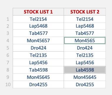
5. Method 1: Highlighting Row Differences with Conditional Formatting

Conditional formatting is a quick and easy way to visually identify differences between two lists. This method is particularly useful when you want to see how many rows have differing values across two columns.

Steps:

1. Select the Columns: Select both columns you want to compare.

2. Go to Conditional Formatting: Go to Home > Conditional Formatting > New Rule.

3. Choose a Rule Type: Select “Use a formula to determine which cells to format”.

4. Enter the Formula: Enter a formula that compares the two cells in the same row. For example, if your data starts in row 2, and you are comparing column A and column B, use the formula: =A2<>B2.

5. Set the Format: Click the “Format” button and choose the desired formatting (e.g., fill color, font color).

6. Click OK: Click “OK” to apply the conditional formatting rule.

This will highlight all cells where the values in the corresponding rows of the two columns are different.

Advantages:

• Visually highlights differences quickly.
• Easy to set up and use.

Disadvantages:

• Doesn’t provide specific information about matches or mismatches.
• Not suitable for large datasets.

6. Method 2: Comparing Rows Using the IF Function

The IF function allows you to compare two lists and return a specific value (e.g., “Match” or “Not a Match”) based on whether the values in the same row are equal.

Steps:

1. Enter the IF Function: In a blank cell, enter the IF function. For example, if you are comparing cells A2 and B2, the formula would be: =IF(A2=B2, "Match", "Not a Match").

2. Drag the Formula: Drag the lower-right corner of the cell downwards to apply the formula to the rest of the rows.

This will display “Match” for rows where the values in the two columns are equal and “Not a Match” for rows where they are different.

Advantages:

• Simple and easy to understand.
• Provides clear “Match” or “Not a Match” results.

Disadvantages:

• Requires an additional column to display the results.
• Doesn’t provide information about the position of matches.

7. Method 3: Leveraging the MATCH Function for List Comparison

The MATCH function is a powerful tool for comparing two lists in Excel to find matches. It searches for a value in a range and returns the position of that value in the range. If the value is not found, it returns #N/A.

Steps:

1. Enter the MATCH Function: In a blank cell, enter the MATCH function. For example, if you want to check if the value in cell A2 exists in column B, the formula would be: =MATCH(A2, B:B, 0).

2. Drag the Formula: Drag the lower-right corner of the cell downwards to apply the formula to the rest of the rows.

This will return the row number in column B where the value from column A is found. If the value is not found, it will return #N/A.

Advantages:

• Identifies the position of matches in the second list.
• Can be used to filter the list based on matches or mismatches.

Disadvantages:

• Returns #N/A for mismatches, which may require additional handling.
• Doesn’t provide information about the value of the matches.

8. Practical Scenarios for List Comparison Using the MATCH Function

8.1. Exact Row Matches with MATCH Function

Identifying exact row matches is essential for many data management tasks. The MATCH function helps you quickly pinpoint the location of a specific value within a column.

Example:

Suppose you have a list of employee names in column A and their corresponding employee IDs in column B. You want to find the row number for the employee named “Alice”. You can use the MATCH function as follows:

=MATCH("Alice", A:A, 0)

This formula will return the row number where “Alice” is found in column A. You can then use this row number to retrieve other information about Alice, such as her employee ID, using the INDEX function.

8.2. Identifying Mismatches Between Lists

Finding mismatches between lists is crucial for maintaining data integrity. By combining the MATCH function with the ISNA function, you can easily identify values in one list that are not present in another.

Example:

You have two lists of product SKUs: one representing your current inventory (column A) and another representing your sales orders (column B). To find which SKUs in your inventory are not present in your sales orders, use the following formula:

=ISNA(MATCH(A2, B:B, 0))

This formula will return TRUE if the SKU in cell A2 is not found in column B, indicating a mismatch. You can then filter the list to show only the mismatches.

9. Tips and Tricks for Optimizing Your MATCH Formulas

9.1. Handling Case-Sensitivity Issues in List Comparison

The MATCH function is case-insensitive by default, which means it treats “Apple” and “apple” as the same value. If you need to perform a case-sensitive comparison, you can combine the MATCH function with the EXACT function.

Example:

To perform a case-sensitive comparison of values in column A and column B, use the following formula:

=MATCH(TRUE, EXACT(A2, B:B), 0)

This formula will return the row number where the value in cell A2 matches the value in column B exactly, including case.

9.2. Avoiding Common Errors with MATCH Function

The most common error encountered when using the MATCH function is the #N/A error, which indicates that the lookup value was not found in the lookup array. To avoid this error, ensure that:

• The lookup value is spelled correctly and matches the format of the values in the lookup array.
• The lookup array is a single column or row.
• The match type is set to 0 for an exact match.
• The lookup value actually exists in the lookup array.

If you still encounter the #N/A error, you can use the IFERROR function to handle it gracefully. For example:

=IFERROR(MATCH(A2, B:B, 0), "Not Found")

This formula will return “Not Found” instead of #N/A if the value in cell A2 is not found in column B.

10. Advanced Techniques for List Comparison

10.1. Comparing Multiple Columns

Sometimes, you need to compare multiple columns to determine if a row is a match. You can use the AND function in combination with the IF function to achieve this.

Example:

Suppose you have two tables with customer data, and you want to identify customers who have the same first name, last name, and email address. You can use the following formula:

=IF(AND(A2=D2, B2=E2, C2=F2), "Match", "Not a Match")

This formula will return “Match” if the values in columns A, B, and C of the first table match the values in columns D, E, and F of the second table, respectively.

10.2. Using Array Formulas for Complex Comparisons

Array formulas can be used to perform complex comparisons that involve multiple criteria or conditions.

Example:

Suppose you want to find all the products in your inventory that have a price greater than $100 and a quantity less than 10. You can use the following array formula:

=SUM((A2:A100>100)*(B2:B100<10))

This formula will return the number of products that meet both criteria. To enter an array formula, you need to press Ctrl+Shift+Enter instead of just Enter.

11. Alternatives to MATCH Function for List Comparison

While the MATCH function is a powerful tool for comparing lists in Excel, there are several alternatives that you can use depending on your specific needs.

11.1. VLOOKUP

VLOOKUP searches for a value in the first column of a range and returns a value from the same row in another column. It can be used to determine if a value from one list exists in another and to retrieve additional information about the match.

Example:

To check if the value in cell A2 exists in column D and return the corresponding value from column E, use the following formula:

=VLOOKUP(A2, D:E, 2, FALSE)

This formula will return the value from column E if the value in cell A2 is found in column D. If the value is not found, it will return #N/A.

11.2. INDEX and MATCH Combination

The INDEX and MATCH functions can be combined to perform more flexible lookups than VLOOKUP. INDEX returns the value at a specific location in a range, and MATCH provides the row or column number.

Example:

To find the value in column E that corresponds to the value in cell A2, use the following formula:

=INDEX(E:E, MATCH(A2, D:D, 0))

This formula will return the value from column E that is in the same row as the value in cell A2 in column D.

11.3. XLOOKUP

XLOOKUP is a newer function that combines the features of VLOOKUP and INDEX/MATCH and offers several advantages, such as the ability to look in any direction and handle missing values more gracefully.

Example:

To find the value in column E that corresponds to the value in cell A2, use the following formula:

=XLOOKUP(A2, D:D, E:E)

This formula will return the value from column E that corresponds to the value in cell A2 in column D. If the value is not found, it will return #N/A.

12. Using Power Query for Advanced List Comparison

Power Query (Get & Transform Data) is a powerful data transformation tool built into Excel. It can be used to perform advanced list comparisons, especially when dealing with large datasets or complex criteria.

Steps:

1. Load Data into Power Query: Select the data you want to compare and go to Data > From Table/Range.

2. Merge Queries: In the Power Query Editor, go to Home > Merge Queries.

3. Choose Tables and Columns: Select the two tables you want to merge and choose the columns to match on.

4. Select Join Kind: Choose the join kind that suits your needs (e.g., Left Outer, Right Outer, Inner).

5. Expand Columns: Expand the columns from the merged table that you want to include in the result.

6. Load the Result: Go to Home > Close & Load to load the result into a new worksheet.

Power Query allows you to perform complex list comparisons with ease and efficiency, even when dealing with large and complex datasets.

13. Automating List Comparisons with VBA Macros

For repetitive list comparison tasks, you can automate the process using VBA macros.

Example:

The following VBA code compares two columns and highlights the differences:

Sub CompareLists()
  Dim i As Long
  Dim LastRow As Long

  ' Get the last row of data in column A
  LastRow = Cells(Rows.Count, "A").End(xlUp).Row

  ' Loop through each row in column A
  For i = 2 To LastRow
    ' Compare the value in column A with the value in column B
    If Cells(i, "A").Value <> Cells(i, "B").Value Then
      ' Highlight the cell in column A if the values are different
      Cells(i, "A").Interior.Color = vbYellow
    End If
  Next i
End Sub

This code loops through each row in column A and compares the value with the value in column B. If the values are different, it highlights the cell in column A in yellow.

14. Best Practices for Efficient List Comparison

To ensure efficient and accurate list comparison, follow these best practices:

• Clean Your Data: Remove any unnecessary spaces, special characters, or formatting inconsistencies.
• Use Consistent Formatting: Ensure that the data in both lists is formatted consistently.
• Sort Your Data: Sorting the data can make it easier to identify matches and mismatches.
• Use Absolute Cell References: When using formulas, use absolute cell references (e.g., $A$2) to prevent errors when dragging the formula.
• Test Your Formulas: Always test your formulas on a small sample of data before applying them to the entire dataset.
• Document Your Process: Document the steps you took to compare the lists so that you can easily repeat the process in the future.

15. Advanced Tips and Tricks for Speeding Up List Comparison

• Use the Evaluate Formula Tool: The Evaluate Formula tool can help you understand how Excel is calculating your formulas and identify any errors.

• Disable Automatic Calculation: Disabling automatic calculation can speed up the performance of your formulas, especially when working with large datasets.

• Use the Watch Window: The Watch Window allows you to monitor the values of specific cells or formulas as you make changes to your worksheet.

• Use the Immediate Window: The Immediate Window can be used to test VBA code and debug macros.

16. FAQ: Frequently Asked Questions About List Comparison in Excel

16.1. How Do I Use MATCH to Compare Two Columns in Excel?

To use MATCH to compare two columns in Excel, you would use the function to search for a specific item from the first column within the second column. Here’s what you’d do in a nutshell: Set your lookup value to be a cell reference from the first column. This is the value MATCH will look for in the second column. Define the lookup array to be the range of the second column. Specify the match type as 0 for an exact match, which is often what you’re after when comparing columns. Apply the formula across all relevant cells in the first column to check for each value’s presence in the second column.

Here’s a quick formula example, assuming you’re comparing Column A to Column B: =MATCH(A2, B:B, 0)

Drag this formula down along Column A, and you’ll see results indicating where in Column B each value of Column A can be found, or #N/A if there’s no match.

16.2. Can I Find Partial Matches with the MATCH Function in Excel?

Yes, even though the MATCH function itself looks for exact matches by default, you can gear up Excel to seek out partial matches. This can be a game-changer when working with data that contains similar but not identical entries. Cue the wildcard characters, the asterisk (*) and the question mark (?), for partial matches.

For instance, if you’re comparing company names, and you want to find “JPMorgan” even when it’s listed as “JPMorgan Chase,” an asterisk can help: =MATCH("*"&"JPMorgan"&"*", Range, 0)

The asterisks tell Excel to find any cell where “JPMorgan” appears, surrounded by any number of characters. Just remember, MATCH and wildcards can be a slightly more complex combination, so be extra mindful of what you’re looking for to prevent inaccurate matches.

16.3. What Are Some Alternatives to the MATCH Function for Comparing Lists?

While the MATCH function is quite the tool for comparing lists in Excel, one size doesn’t fit all in the data analysis wardrobe. Depending on the task at hand, VLOOKUP, INDEX, and the newer XLOOKUP might better suit your needs.

VLOOKUP, the veteran, takes a lookup value and scans down the first column of a specified range to return a value from the same row. It’s great when you need more than just the position and want the actual data. However, it’s limited to searching only to the right.

INDEX and MATCH can be paired for more flexibility, with INDEX returning the value at a specific location in a range, and MATCH providing the row or column number.

And then there’s XLOOKUP, Excel’s latest couture, designed to eliminate VLOOKUP’s limitations. XLOOKUP can look in any direction—up, down, left, or right—and it handles missing values more gracefully.

Picking the right function is all about the context of your comparison chore. Quick matches? Go with MATCH. Data retrieval? VLOOKUP or INDEX with MATCH. The utmost flexibility? XLOOKUP is your ace.

17. Conclusion: Mastering List Comparison in Excel

Comparing two lists in Excel to find matches doesn’t have to be a daunting task. By understanding the various methods and techniques available, you can streamline the process, reduce errors, and gain valuable insights from your data. Whether you’re using conditional formatting, the IF function, the MATCH function, or more advanced techniques like Power Query and VBA macros, the key is to choose the method that best suits your specific needs and data. Remember to clean your data, use consistent formatting, and test your formulas to ensure accuracy.

Are you ready to take your Excel skills to the next level? Visit COMPARE.EDU.VN today to explore more in-depth tutorials, practical examples, and expert advice on data analysis and list comparison. Let us help you make informed decisions and unlock the full potential of your data. Contact us at 333 Comparison Plaza, Choice City, CA 90210, United States, or reach out via Whatsapp at +1 (626) 555-9090. You can also visit our website at compare.edu.vn for more information.