How To Compare Two Lists In Excel For Matches is a common challenge, and COMPARE.EDU.VN is here to provide solutions. This guide explores different Excel functions and features to identify matching entries, highlight differences, and streamline your data comparison tasks. Find the best approach for your needs with these list comparison techniques.
1. Highlight Row Difference Using Conditional Formatting
You can quickly identify differences in values between rows using Excel’s conditional formatting feature. This method is useful for getting an overview of how many rows have differing values across two columns.
In this example, we have two lists in Column A and Column B. Here’s how to highlight the row differences:
1.1 Select the Columns
Start by selecting both columns containing the lists you want to compare.
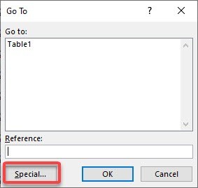
1.2 Open the Go To Special Dialog
Navigate to Home > Find & Select > Go To Special. Alternatively, press Ctrl + G and then click Special to open the “Go To Special” dialog box.
1.3 Select Row Difference
In the “Go To Special” dialog, choose Row Difference and click OK.
1.4 Observe the Highlighted Differences
Excel will highlight the values in the second list (Column B) that do not match the corresponding values in the first list (Column A).
1.5 Optional: Mark Cells with Color
To further emphasize the differences, you can change the font color of the highlighted cells. Go to Home > Font Color and select Red (or any color of your choice).
This method provides a visual way to spot the differences between your two lists.
2. Compare Rows Using the IF Function
The IF function is a versatile tool for comparing two lists in Excel and determining if values in the same row match. It returns TRUE if the values match and FALSE if they don’t. You can also customize the output to display text like “Match” or “Not a Match.”
Here’s how to compare lists using the IF function:
2.1 Enter the IF Function
In a blank cell, enter the IF function: =IF(
2.2 Define the Logical Test
The first argument of the IF function is the logical test, which is the condition you want to check. In this case, we want to check if the value in one cell is equal to the value in another cell. For example, if you’re comparing cell D12 to cell C12, your formula would start like this: =IF(D12=C12,
2.3 Define the Value if True
The second argument is the value that should be displayed if the condition is TRUE. In this example, we want to display the text “Match” if the values are equal. So, the formula would now look like this: =IF(D12=C12,"Match",
2.4 Define the Value if False
The third argument is the value that should be displayed if the condition is FALSE. Here, we want to display “Not a Match” if the values are not equal: =IF(D12=C12,"Match","Not a Match")
2.5 Apply the Formula to the Rest of the Cells
Drag the lower right corner of the cell containing the formula downwards to apply it to the rest of the rows. This will automatically compare the corresponding cells in each row and display “Match” or “Not a Match” accordingly.
3. Compare Lists Using the MATCH Function
The MATCH function is an invaluable tool for comparing two lists in Excel for matches. It tells you the position of an item in a range.
3.1 Understanding the MATCH Function
The basic syntax of the MATCH function is:
=MATCH(lookup_value, lookup_array, [match_type])
- lookup_value: The value you want to find.
- lookup_array: The range of cells where you want to search.
- match_type: (Optional) Specifies how MATCH should find the lookup_value. Use 0 for an exact match.
3.2 Practical Application
Imagine you have two lists and you want to know if a specific item in List1 exists in List2. The MATCH function can verify if a cell’s item in List1 exists in List2. It will return the row position of that item in List2, confirming its existence. If you get a #N/A error, it means the item does not exist in List2.
Here are our two lists:
3.3 Steps to Use the MATCH Function
3.3.1 Enter the MATCH Function
In a blank cell, enter the MATCH function: =MATCH(
3.3.2 Define the Lookup Value
Select the cell containing the List1 value, as this is what we want to check against List2: =MATCH(C12,
3.3.3 Define the Lookup Array
Select the entire List2 range you want to check against. Ensure you press F4 to make it an absolute reference, which prevents the cell references from changing when you copy the formula: =MATCH(C12, list2!$C$12:$C$21,
3.3.4 Define the Match Type
Since we want an exact match, specify 0 as the match type: =MATCH(C12, list2!$C$12:$C$21, 0)
3.3.5 Apply the Formula to the Remaining Cells
Drag the lower right corner of the cell downwards to apply the formula to the rest of the cells.
3.4 Interpreting the Results
Excel will return the row number where the item exists in List2. For example, if the formula returns 9, it means the item from List1 exists in List2 in row 9. If the item does not exist, the formula will return #N/A.
4. Practical Scenarios for List Comparison
Comparing lists in Excel is not just a theoretical exercise; it has numerous real-world applications. Let’s explore some practical scenarios where these techniques can be incredibly useful.
4.1 Exact Row Matches with MATCH Function
Identifying where exact values line up in lists is crucial in many scenarios. The MATCH function can be used to pinpoint a value’s position within a column. For example, you can link data across different sheets.
Suppose you have a list of employees in one column and their unique IDs in another. To find out in which row “Jamie” is mentioned, use MATCH to get their row number. This positional number allows you to use other Excel functions to retrieve additional data associated with Jamie.
Remember to use 0 as the third argument for an exact match. This ensures you get an accurate result.
Here’s an example:
=MATCH("Jamie", A2:A100, 0)
4.2 Identifying Mismatches Between Lists
Ensuring that two sets of data are in harmony is a top priority. Excel’s MATCH function helps you catch any discrepancies. Identifying mismatches between lists means finding what’s in one list that’s not in the other.
For example, you might be auditing inventory or ensuring your email list hasn’t missed any subscribers. By using MATCH alongside an error-catching function like ISNA, you’re equipped to flag discrepancies.
Here’s an example:
=ISNA(MATCH(value from List A, Range of List B, 0))
This formula returns TRUE when a value from List A is missing in List B, indicating a mismatch.
5. Tips and Tricks for Optimizing Your MATCH Formulas
To get the most out of the MATCH function, here are some tips and tricks that can help you optimize your formulas and avoid common pitfalls.
5.1 Handling Case-Sensitivity Issues in List Comparison
Excel’s MATCH function does not distinguish between uppercase and lowercase letters, which can be problematic in certain datasets. If you need to treat “Data” and “data” as unique entries, you’ll need a workaround to make your list comparison case-sensitive.
You can transform MATCH into a detail-oriented tool by partnering it with the EXACT function, which strictly compares text, taking the case of each letter into account. The combined formula looks like this:
=MATCH(TRUE, EXACT(Cell Range, "Your Text"), 0)
If “Your Text” does not match the exact case in the cell range, MATCH will not find it. Note that this can be an array formula, so press Ctrl+Shift+Enter if you’re not using Excel 365 or later.
5.2 Avoiding Common Errors with MATCH Function
When using MATCH, you might encounter the dreaded #N/A error, which means Excel can’t find what you’re looking for. Here are some tips to avoid this error:
- Check Your Lookup Value: Ensure that your lookup value is spelled correctly and doesn’t contain any extra spaces.
- Scrutinize the Lookup Array: The range should be a single column or row. Also, remember to lock your array with absolute cell references (e.g.,
$A$1:$A$100) if your formula needs to stay constant across multiple cells. - Ensure Correct Match Type: Use 0 for an exact match to avoid unintentional approximate matches.
6. FAQ: Frequently Asked Questions
Let’s address some common questions about using the MATCH function for list comparison in Excel.
6.1 How Do I Use MATCH to Compare Two Columns in Excel?
To compare two columns using MATCH, you direct the function to search for a specific item from the first column within the second column.
Here’s what you do:
- Set your lookup value to be a cell reference from the first column.
- Define the lookup array as the range of the second column.
- Specify the match type as 0 for an exact match.
- Apply the formula across all relevant cells in the first column.
Here’s a formula example for comparing Column A to Column B:
=MATCH(A2, B:B, 0)
Drag this formula down along Column A to see the results indicating where in Column B each value of Column A can be found, or #N/A if there’s no match.
6.2 Can I Find Partial Matches with the MATCH Function in Excel?
Yes, although MATCH looks for exact matches by default, you can use wildcard characters to find partial matches. The asterisk (*) and the question mark (?) can be used for this purpose.
For example, if you’re comparing company names and want to find “JPMorgan” even when it’s listed as “JPMorgan Chase,” use an asterisk:
=MATCH("*"&"JPMorgan"&"*", Range, 0)
The asterisks tell Excel to find any cell where “JPMorgan” appears, surrounded by any number of characters. Be mindful when using wildcards to ensure accurate matches.
6.3 What Are Some Alternatives to the MATCH Function for Comparing Lists?
While MATCH is a useful tool, VLOOKUP, INDEX, and XLOOKUP can also be used for comparing lists in Excel, depending on your needs.
- VLOOKUP: Takes a lookup value and scans down the first column of a specified range to return a value from the same row. It’s great when you need more than just the position and want the actual data, but it’s limited to searching only to the right.
- INDEX and MATCH: Can be paired for more flexibility, with INDEX returning the value at a specific location in a range, and MATCH providing the row or column number.
- XLOOKUP: Excel’s latest function, designed to eliminate VLOOKUP’s limitations. XLOOKUP can look in any direction—up, down, left, or right—and it handles missing values more gracefully.
Choosing the right function depends on the specific context of your comparison task.
7. Conclusion: Streamlining List Comparisons in Excel
Comparing two lists in Excel for matches can be a straightforward process with the right tools and techniques. Whether you use conditional formatting for visual cues, the IF function for simple matches, or the MATCH function for more complex scenarios, Excel offers a variety of methods to suit your needs.
At COMPARE.EDU.VN, we understand the importance of making informed decisions based on accurate data comparisons. That’s why we’ve provided these detailed explanations and practical examples to help you master list comparisons in Excel.
Are you struggling to compare multiple options and make the right choice? Visit COMPARE.EDU.VN today for detailed and objective comparisons that simplify your decision-making process. Our comprehensive comparisons can help you save time and ensure you make the best choice for your needs.
Contact us:
Address: 333 Comparison Plaza, Choice City, CA 90210, United States
Whatsapp: +1 (626) 555-9090
Website: compare.edu.vn

