How to Compare Two Lists in Excel and Pull Differences

Comparing data in Excel is a common task, especially when dealing with two lists. Whether you need to find matches, highlight differences, or extract unique values, Excel offers various techniques. This guide provides a comprehensive overview of How To Compare Two Lists In Excel And Pull Differences, using formulas, conditional formatting, and other helpful tools.

Comparing Two Columns Row-by-Row Using Formulas

The IF function is a powerful tool for comparing data row by row. Here’s how to use it:

Finding Matches and Differences

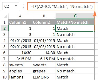
1. Basic Comparison: To compare cells A2 and B2, enter the following formula in another column (e.g., C2): =IF(A2=B2,"Match","No match"). This formula returns “Match” if the cells are identical and “No match” if they differ.

2. Case-Sensitive Comparison: For case-sensitive matching, use the EXACT function: =IF(EXACT(A2,B2),"Match","No match").

3. Copy Down: Drag the fill handle (the small square at the bottom right of the cell) down to apply the formula to all rows.

Comparing Multiple Columns in the Same Row

1. Matching All Cells: To find rows where all cells are identical, use the AND function with IF: =IF(AND(A2=B2,A2=C2),"Full match",""). Alternatively, use COUNTIF: =IF(COUNTIF($A2:$E2,$A2)=5,"Full match",""), where 5 represents the number of columns.

2. Matching Any Two Cells: To find rows where at least two cells match, use the OR function with IF: =IF(OR(A2=B2,B2=C2,A2=C2),"Match",""). For multiple columns, consider using a combination of COUNTIF functions.

Identifying Unique Values in Two Lists

To identify values present in one list but not the other (List A in column A, List B in column B), use these methods:

1. COUNTIF: =IF(COUNTIF($B:$B, $A2)=0, "No match in B", ""). This formula returns “No match in B” if the value in A2 is not found in column B.

2. MATCH and ISERROR: =IF(ISERROR(MATCH($A2,$B$2:$B$10,0)),"No match in B",""). This formula uses MATCH to search for A2 in B2:B10. ISERROR checks if MATCH returns an error (no match found).

3. Array Formula: {=IF(SUM(--($B$2:$B$10=$A2))=0,"No match in B","")}. Remember to press Ctrl + Shift + Enter for array formulas. This formula sums instances of A2 in B2:B10. If the sum is 0, it means no match is found.

Highlighting Matches and Differences with Conditional Formatting

Conditional formatting visually emphasizes differences and matches:

1. Highlighting Row Matches/Differences: Select the cells, go to Conditional Formatting > New Rule… > Use a formula to determine which cells to format. For matches in the same row, use =$A2=$B2. For differences, use =$A2<>$B2.

2. Highlighting Unique Values: To highlight unique values in List A, use =COUNTIF($B$2:$B$5,$A2)=0. For List B, use =COUNTIF($A$2:$A$6,$C2)=0.

3. Highlighting Duplicate Values: Use =COUNTIF($B$2:$B$5,$A2)>0 for List A and =COUNTIF($A$2:$A$6,$C2)>0 for List B.

Comparing Multiple Columns and Highlighting Row Differences

1. Highlighting Row Matches: Use conditional formatting with formulas like =AND($A2=$B2,$A2=$C2) or =COUNTIF($A2:$C2,$A2)=3.

2. Highlighting Row Differences using Go To Special: Select the range, go to Home > Find & Select > Go To Special…, select Row differences, and click OK. This highlights cells differing from the active cell in each row. You can then apply fill color.

Conclusion

Excel provides a robust toolkit for comparing lists and identifying differences. By mastering these techniques, you can efficiently analyze data and extract meaningful insights. Whether you prefer using formulas, conditional formatting, or specialized add-ins, Excel offers a solution for your comparison needs.