How to Compare Two Excel Workbooks Using VLOOKUP

Comparing two Excel workbooks can be a daunting task, but with the VLOOKUP function, it becomes significantly easier. At COMPARE.EDU.VN, we provide you with the tools and knowledge to streamline this process, ensuring accuracy and efficiency in your data analysis. Discover how to use VLOOKUP and related techniques to reconcile data discrepancies and maintain data integrity. Explore other methods to compare Excel spreadsheets to make the best choice.

Table of Contents

1. Understanding the Need to Compare Excel Workbooks
2. Setting Up Your Data for Comparison
3. Using VLOOKUP: A Step-by-Step Guide
   • 3. 1 VLOOKUP Syntax and Explanation
   • 3. 2 Handling Missing Values with IFERROR
   • 3. 3 Using XLOOKUP as an Alternative
4. Reconciling Values Using IF Statements
5. Conditional Formatting for Quick Identification
6. Advanced Techniques for Excel Workbook Comparison
   • 6. 1 Using Excel’s Built-in Compare Feature
   • 6. 2 Leveraging Power Query for Data Comparison
   • 6. 3 Using VBA for Complex Comparisons
7. Best Practices for Comparing Excel Workbooks
8. Troubleshooting Common Issues
9. Real-World Applications of Excel Workbook Comparison
10. COMPARE.EDU.VN: Your Partner in Data Analysis
11. Frequently Asked Questions (FAQs)

1. Understanding the Need to Compare Excel Workbooks

In today’s data-driven world, businesses often deal with multiple versions of Excel workbooks. These might contain customer data, financial records, inventory lists, or any other critical information. Comparing these workbooks is essential for several reasons:

• Data Reconciliation: Ensuring that data across different workbooks is consistent and accurate.
• Identifying Discrepancies: Spotting errors, omissions, or inconsistencies that could lead to incorrect decisions.
• Auditing: Verifying that changes made to data are tracked and justified.
• Merging Data: Combining data from multiple sources into a unified, comprehensive dataset.

Whether you are an accountant, data analyst, project manager, or business owner, the ability to compare Excel workbooks efficiently is a valuable skill. At COMPARE.EDU.VN, we aim to provide you with the knowledge and tools to master this skill, ensuring you can make informed decisions based on reliable data. To maintain data integrity, consider techniques like VLOOKUP.

2. Setting Up Your Data for Comparison

Before you can start comparing Excel workbooks, you need to ensure that your data is properly structured. Here are some essential steps to follow:

1. Organize Your Workbooks: Make sure each workbook contains the data you want to compare. Open both workbooks simultaneously.
2. Identify Unique Identifiers: Choose a column that contains unique identifiers, such as Customer ID, Product Code, or Invoice Number. This column will serve as the basis for your comparison.
3. Ensure Data Consistency: Verify that the data types and formats in the columns you want to compare are consistent across both workbooks. For example, ensure that dates are formatted the same way and that numerical values are stored as numbers, not text.
4. Create Backup Copies: Always create backup copies of your original workbooks before making any changes. This ensures that you can revert to the original data if something goes wrong.
5. Understand Your Data: Familiarize yourself with the structure and content of each workbook. Identify the columns you need to compare and understand the relationships between them.

By taking these preliminary steps, you can ensure that your data is ready for comparison, setting the stage for accurate and efficient analysis. Ensure the accuracy of each sheet before running a function like VLOOKUP.

3. Using VLOOKUP: A Step-by-Step Guide

VLOOKUP (Vertical Lookup) is a powerful Excel function that allows you to search for a value in one column and return a corresponding value from another column in the same row. It’s particularly useful for comparing data across two Excel workbooks. Here’s a step-by-step guide on how to use VLOOKUP for this purpose:

Step 1: Open Both Excel Workbooks

Make sure both Excel workbooks you want to compare are open on your computer. This will allow you to reference the data from one workbook in the other.

Step 2: Identify the Common Identifier

Identify a column that is common to both workbooks, such as a Customer ID, Product Code, or Invoice Number. This column will be used as the lookup value.

Step 3: Choose a Target Workbook

Decide which workbook will be the primary one where you will enter the VLOOKUP formula. This is the workbook where you will see the comparison results.

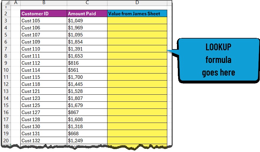
Step 4: Insert a New Column

In the target workbook, insert a new column next to the column containing the common identifier. This new column will hold the results of the VLOOKUP formula.

Step 5: Enter the VLOOKUP Formula

In the first cell of the new column, enter the VLOOKUP formula. The syntax for VLOOKUP is as follows:

=VLOOKUP(lookup_value, table_array, col_index_num, [range_lookup])

• lookup_value: The value you want to search for (e.g., the Customer ID).
• table_array: The range of cells in the second workbook where you want to search for the lookup value and retrieve the corresponding value.
• col_index_num: The column number in the table_array from which you want to retrieve the value.
• [range_lookup]: Optional. Specify FALSE for an exact match or TRUE for an approximate match. It’s generally recommended to use FALSE for accurate comparisons.

Here’s an example of how the VLOOKUP formula might look:

=VLOOKUP(A2,'[Workbook2.xlsx]Sheet1'!$A:$B,2,FALSE)

In this example:

• A2 is the lookup value (e.g., the Customer ID in the first row of the target workbook).
• '[Workbook2.xlsx]Sheet1'!$A:$B is the range in the second workbook where you want to search for the Customer ID and retrieve the corresponding value.
• 2 is the column number in the second workbook from which you want to retrieve the value (e.g., the second column, which might contain the Customer Name).
• FALSE specifies that you want an exact match.

Step 6: Apply the Formula to the Entire Column

Click and drag the fill handle (the small square at the bottom-right corner of the cell) down to apply the VLOOKUP formula to the entire column. This will populate the column with the corresponding values from the second workbook.

Step 7: Handle Errors

If VLOOKUP doesn’t find a match, it will return the #N/A error. You can handle this error using the IFERROR function to display a more user-friendly message, such as “Not Found”.

=IFERROR(VLOOKUP(A2,'[Workbook2.xlsx]Sheet1'!$A:$B,2,FALSE),"Not Found")

Step 8: Compare the Values

Now that you have the corresponding values from the second workbook in the target workbook, you can compare them to the values in the target workbook. Use the IF function to create a new column that indicates whether the values match or not.

=IF(B2=C2,"Match","Mismatch")

In this example:

• B2 is the value from the target workbook.
• C2 is the value retrieved from the second workbook using VLOOKUP.
• If the values match, the formula will display “Match”; otherwise, it will display “Mismatch”.

Step 9: Use Conditional Formatting (Optional)

To quickly identify the mismatches, you can use conditional formatting to highlight the rows where the values don’t match.

1. Select the column containing the “Match” or “Mismatch” results.
2. Go to Home > Conditional Formatting > Highlight Cells Rules > Equal To.
3. Enter “Mismatch” in the dialog box and choose a formatting style (e.g., red fill).
4. Click OK.

Now, all the rows where the values don’t match will be highlighted, making it easy to spot discrepancies.

By following these steps, you can effectively use VLOOKUP to compare data across two Excel workbooks, identify mismatches, and ensure data accuracy.

3.1 VLOOKUP Syntax and Explanation

To fully leverage VLOOKUP, it’s essential to understand its syntax and components. The VLOOKUP function has four arguments:

• Lookup_value: The value you want to search for. This is typically a unique identifier like a product ID or customer number.
• Table_array: The range of cells in which to search for the lookup value. The lookup value should be in the first column of this range.
• Col_index_num: The column number within the table_array that contains the value you want to return.
• Range_lookup: A logical value that specifies whether you want to find an exact match (FALSE) or an approximate match (TRUE). It’s generally safer to use FALSE for accurate comparisons.

For example, if you want to find the price of a product in a table, you would use the product ID as the lookup_value, the table containing the product IDs and prices as the table_array, and the column number containing the prices as the col_index_num.

3.2 Handling Missing Values with IFERROR

One common issue when using VLOOKUP is encountering missing values. When VLOOKUP cannot find a match, it returns the #N/A error. To handle this, you can use the IFERROR function, which allows you to specify a value to return if an error occurs.

For example:

=IFERROR(VLOOKUP(A2,Sheet2!A:B,2,FALSE),"Value Not Found")

This formula will return “Value Not Found” if the VLOOKUP function returns an error, indicating that the lookup value was not found in the specified range.

3.3 Using XLOOKUP as an Alternative

Excel 365 offers an alternative to VLOOKUP called XLOOKUP. XLOOKUP is more flexible and overcomes some of the limitations of VLOOKUP. Here are some advantages of using XLOOKUP:

• No Column Insertion: XLOOKUP doesn’t require the lookup column to be the leftmost column in the table array.
• Handles Missing Values: XLOOKUP has a built-in argument to handle missing values, eliminating the need for IFERROR.
• Better Performance: XLOOKUP is generally faster and more efficient than VLOOKUP.

Here’s an example of how to use XLOOKUP:

=XLOOKUP(A2,Sheet2!A:A,Sheet2!B:B,"Value Not Found")

In this example:

• A2 is the lookup value.
• Sheet2!A:A is the range containing the lookup values.
• Sheet2!B:B is the range containing the return values.
• "Value Not Found" is the value to return if no match is found.

Using XLOOKUP can simplify your formulas and improve the accuracy and efficiency of your comparisons.

4. Reconciling Values Using IF Statements

Once you’ve used VLOOKUP to retrieve corresponding values from the second workbook, you need to reconcile these values to identify any discrepancies. The IF function is invaluable for this purpose.

Here’s how to use the IF function to compare values:

=IF(A2=B2,"Match","Mismatch")

In this formula:

• A2 is the value from the first workbook.
• B2 is the value retrieved from the second workbook using VLOOKUP.
• If the values are equal, the formula returns “Match”; otherwise, it returns “Mismatch”.

You can also use nested IF statements to handle more complex scenarios. For example, you might want to check if a value is within a certain tolerance range.

Here’s an example:

=IF(ABS(A2-B2)<10,"Match within Tolerance","Mismatch")

This formula checks if the absolute difference between the two values is less than 10. If it is, the formula returns “Match within Tolerance”; otherwise, it returns “Mismatch”.

By using IF statements, you can easily identify and categorize discrepancies between your Excel workbooks, enabling you to focus on the most critical issues.

5. Conditional Formatting for Quick Identification

Conditional formatting is a powerful Excel feature that allows you to highlight cells based on specific criteria. This can be incredibly useful for quickly identifying discrepancies between two Excel workbooks.

Here’s how to use conditional formatting:

1. Select the Range: Select the range of cells you want to format.
2. Open Conditional Formatting: Go to Home > Conditional Formatting.
3. Create a New Rule: Choose New Rule.
4. Select Rule Type: Select Use a formula to determine which cells to format.
5. Enter the Formula: Enter a formula that evaluates to TRUE when the cell should be formatted.

For example, to highlight mismatches, you can use the following formula:

=$C2="Mismatch"

In this formula, $C2 refers to the column containing the “Match” or “Mismatch” results from the IF function. The $ sign ensures that the column reference remains fixed when the formatting is applied to other cells.

1. Set the Format: Click on Format and choose the formatting style you want to apply (e.g., red fill).
2. Click OK: Click OK to apply the conditional formatting rule.

Now, all the cells where the values don’t match will be highlighted, making it easy to spot discrepancies. You can add multiple conditional formatting rules to highlight different types of discrepancies.

6. Advanced Techniques for Excel Workbook Comparison

While VLOOKUP and IF statements are effective for basic comparisons, more complex scenarios may require advanced techniques. Here are some additional methods to consider:

6.1 Using Excel’s Built-in Compare Feature

Excel has a built-in feature that allows you to compare two workbooks directly. To use this feature:

1. Open Both Workbooks: Open both Excel workbooks you want to compare.
2. Go to View Tab: Click on the View tab in the Excel ribbon.
3. Click Compare: In the Window group, click Compare Side by Side.
4. Synchronize Scrolling: If you want to scroll both workbooks simultaneously, click on Synchronous Scrolling in the Window group.

Excel will display both workbooks side by side, highlighting the differences between them. This feature is useful for visually identifying discrepancies and understanding the changes made to the workbooks.

6.2 Leveraging Power Query for Data Comparison

Power Query is a powerful data transformation and analysis tool built into Excel. It allows you to import data from multiple sources, clean and transform it, and perform complex comparisons.

Here’s how to use Power Query for data comparison:

1. Import Data: Import the data from both Excel workbooks into Power Query. Go to Data > Get & Transform Data > From File > From Workbook.
2. Transform Data: Use Power Query’s transformation tools to clean and standardize the data. This might involve renaming columns, changing data types, or removing duplicates.
3. Merge Queries: Merge the two queries based on a common identifier. Click on Home > Merge Queries.
4. Expand Columns: Expand the columns from the second query that you want to compare.
5. Add a Conditional Column: Add a conditional column to compare the values from the two queries. Click on Add Column > Conditional Column.
6. Load the Data: Load the transformed data back into Excel. Click on Home > Close & Load.

Power Query provides a flexible and powerful way to compare data from multiple sources, perform complex transformations, and identify discrepancies.

6.3 Using VBA for Complex Comparisons

For highly customized comparisons, you can use Visual Basic for Applications (VBA). VBA is a programming language built into Excel that allows you to automate tasks and create custom functions.

Here’s an example of how to use VBA to compare two Excel workbooks:

Sub CompareWorkbooks()

Dim wb1 As Workbook, wb2 As Workbook
Dim ws1 As Worksheet, ws2 As Worksheet
Dim lastRow As Long, i As Long
Dim id As String, value1 As Variant, value2 As Variant

' Set references to the workbooks and worksheets
Set wb1 = Workbooks("Workbook1.xlsx")
Set wb2 = Workbooks("Workbook2.xlsx")
Set ws1 = wb1.Sheets("Sheet1")
Set ws2 = wb2.Sheets("Sheet1")

' Find the last row with data in the first worksheet
lastRow = ws1.Cells(Rows.Count, "A").End(xlUp).Row

' Loop through each row in the first worksheet
For i = 2 To lastRow ' Assuming data starts from row 2
    ' Get the ID from the first worksheet
    id = ws1.Cells(i, "A").Value

    ' Find the corresponding value in the second worksheet
    value1 = ws1.Cells(i, "B").Value ' Value from Workbook1
    value2 = Application.WorksheetFunction.VLookup(id, ws2.Range("A:B"), 2, False)

    ' Compare the values
    If Not IsError(value2) Then ' Check if VLookup found a match
        If value1 = value2 Then
            ws1.Cells(i, "C").Value = "Match"
        Else
            ws1.Cells(i, "C").Value = "Mismatch"
        End If
    Else
        ws1.Cells(i, "C").Value = "ID Not Found"
    End If
Next i

End Sub

This VBA code iterates through each row in the first workbook, uses VLOOKUP to find the corresponding value in the second workbook, and compares the values. It then writes the results (“Match”, “Mismatch”, or “ID Not Found”) to a new column in the first workbook.

VBA allows you to create highly customized comparison routines tailored to your specific needs.

7. Best Practices for Comparing Excel Workbooks

To ensure accurate and efficient comparisons, follow these best practices:

• Standardize Data: Ensure that the data in both workbooks is standardized and consistent. This includes using consistent data types, formats, and naming conventions.
• Use Unique Identifiers: Always use unique identifiers as the basis for your comparisons. This ensures that you are comparing the correct records.
• Handle Missing Values: Use IFERROR or similar functions to handle missing values gracefully. This prevents errors and ensures that your comparisons are accurate.
• Validate Results: Always validate the results of your comparisons to ensure that they are accurate. This might involve manually reviewing a sample of the results or using additional validation techniques.
• Document Your Process: Document your comparison process, including the steps you took, the formulas you used, and any assumptions you made. This makes it easier to reproduce the results and troubleshoot any issues.
• Regularly Update Your Skills: Stay up-to-date with the latest Excel features and techniques for data comparison. This ensures that you are using the most efficient and effective methods.

8. Troubleshooting Common Issues

When comparing Excel workbooks, you may encounter some common issues. Here are some troubleshooting tips:

• #N/A Errors: This error indicates that VLOOKUP could not find a match. Check that the lookup value exists in the second workbook and that the table_array is specified correctly.
• Incorrect Results: If you are getting incorrect results, double-check your formulas and ensure that you are using the correct column numbers and ranges.
• Performance Issues: If you are working with large workbooks, the comparison process can be slow. Consider using Power Query or VBA to improve performance.
• Data Type Mismatches: Ensure that the data types in the columns you are comparing are consistent. For example, if one column contains numbers formatted as text, convert them to numbers before performing the comparison.
• Hidden Rows or Columns: Make sure there are no hidden rows or columns that might be affecting the comparison results.

9. Real-World Applications of Excel Workbook Comparison

Comparing Excel workbooks has numerous real-world applications across various industries:

• Finance: Reconciling financial statements, comparing budget vs. actual data, and auditing transactions.
• Accounting: Comparing general ledgers, verifying invoices, and reconciling bank statements.
• Supply Chain Management: Comparing inventory lists, tracking orders, and managing shipments.
• Human Resources: Comparing employee records, tracking performance reviews, and managing payroll data.
• Marketing: Comparing sales data, analyzing customer behavior, and tracking campaign performance.
• Healthcare: Comparing patient records, tracking medical supplies, and managing billing data.

In each of these scenarios, the ability to compare Excel workbooks accurately and efficiently is essential for making informed decisions and maintaining data integrity.

10. COMPARE.EDU.VN: Your Partner in Data Analysis

At COMPARE.EDU.VN, we understand the challenges of working with data. That’s why we’re dedicated to providing you with the resources you need to master Excel and other data analysis tools. Whether you’re a beginner or an experienced professional, our comprehensive guides, tutorials, and templates can help you improve your skills and achieve your goals.

We offer a wide range of resources, including:

• Detailed Tutorials: Step-by-step instructions on how to use Excel functions and features.
• Practical Examples: Real-world examples of how to apply Excel to solve common business problems.
• Downloadable Templates: Ready-to-use templates that can save you time and effort.
• Expert Advice: Tips and tricks from experienced data analysts.

Visit COMPARE.EDU.VN today to discover how we can help you unlock the full potential of Excel and transform your data into actionable insights.

For further assistance, you can reach us at:

• Address: 333 Comparison Plaza, Choice City, CA 90210, United States
• WhatsApp: +1 (626) 555-9090
• Website: COMPARE.EDU.VN

11. Frequently Asked Questions (FAQs)

Q1: What is VLOOKUP and how does it work?

VLOOKUP (Vertical Lookup) is an Excel function that searches for a value in the first column of a range and returns a corresponding value from another column in the same row. It is used to compare and reconcile data across different Excel sheets or workbooks.

Q2: How do I handle #N/A errors when using VLOOKUP?

You can use the IFERROR function to handle #N/A errors. The IFERROR function allows you to specify a value to return if the VLOOKUP function returns an error, such as “Value Not Found”.

Q3: What is XLOOKUP and how is it different from VLOOKUP?

XLOOKUP is an alternative to VLOOKUP available in Excel 365. XLOOKUP is more flexible and overcomes some of the limitations of VLOOKUP. It doesn’t require the lookup column to be the leftmost column in the table array, and it has a built-in argument to handle missing values.

Q4: How can I use conditional formatting to highlight discrepancies?

Conditional formatting allows you to highlight cells based on specific criteria. You can use conditional formatting to highlight mismatches by creating a rule that formats cells where the values don’t match.

Q5: What is Power Query and how can it be used for data comparison?

Power Query is a data transformation and analysis tool built into Excel. It allows you to import data from multiple sources, clean and transform it, and perform complex comparisons.

Q6: Can I use VBA to compare Excel workbooks?

Yes, you can use Visual Basic for Applications (VBA) to create custom comparison routines tailored to your specific needs. VBA allows you to automate tasks and create custom functions.

Q7: What are some best practices for comparing Excel workbooks?

Best practices include standardizing data, using unique identifiers, handling missing values, validating results, documenting your process, and regularly updating your skills.

Q8: How can I improve the performance of Excel workbook comparisons?

If you are working with large workbooks, consider using Power Query or VBA to improve performance. Also, ensure that your data is properly indexed and that you are using efficient formulas.

Q9: What are some real-world applications of Excel workbook comparison?

Excel workbook comparison has numerous real-world applications across various industries, including finance, accounting, supply chain management, human resources, marketing, and healthcare.

Q10: Where can I find more resources and support for using Excel for data analysis?

Visit COMPARE.EDU.VN for detailed tutorials, practical examples, downloadable templates, and expert advice on using Excel for data analysis.

By understanding these FAQs and utilizing the resources available at compare.edu.vn, you can master the art of comparing Excel workbooks and make informed decisions based on accurate data.