How to Compare Two Excel Sheets Using Formula

Comparing data across two Excel spreadsheets can be a tedious task. Fortunately, Excel formulas like VLOOKUP and XLOOKUP offer efficient solutions. This tutorial provides a step-by-step guide on How To Compare Two Excel Sheets Using Formulas, ensuring data accuracy and saving valuable time.

Setting Up Your Data

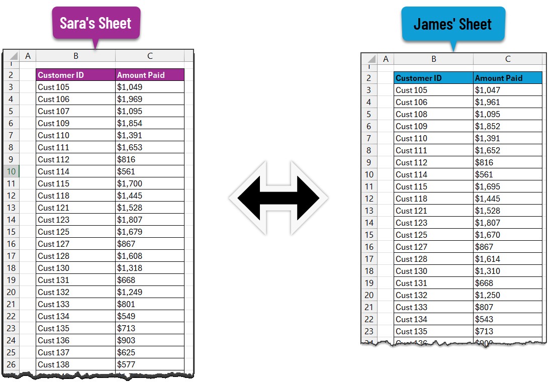
Begin by copying the data from both sources into two separate sheets within the same Excel workbook. Ensure that both datasets have identical column headers, even if the data within the columns differs. A unique identifier column, such as “Customer ID” or “Invoice Number,” is crucial for this comparison process.

Utilizing VLOOKUP for Comparison

Choose Your Starting Sheet: Select the sheet where you want to display the comparison results.
Implement the VLOOKUP Formula: In a new column adjacent to your data, enter the VLOOKUP formula. This formula will search for matching values in the second sheet based on the unique identifier.
```
=VLOOKUP(B3,'Second Sheet'!$B$3:$C$32,2,FALSE)
```
- B3: Represents the cell containing the unique identifier in the current row.
- ‘Second Sheet’!$B$3:$C$32: Specifies the range containing the data in the second sheet, including the unique identifier column and the column you want to compare. The dollar signs ($) make this reference absolute, preventing it from changing when you copy the formula.
- 2: Indicates the column number within the specified range from which to retrieve the corresponding value. In this case, it’s the second column.
- FALSE: Ensures an exact match is required for the lookup.
Using XLOOKUP (Excel 365 and later): If you have Excel 365 or later versions, XLOOKUP offers a more flexible alternative:
```
 =XLOOKUP(B3,'Second Sheet'!$B$3:$B$32,'Second Sheet'!$C$3:$C$32, "ID missing")
```
- “ID missing”: This argument provides a custom message if a matching ID is not found, enhancing clarity.
Apply the Formula: Drag the fill handle (the small square at the bottom right of the cell) down to apply the formula to all rows.

Reconciling the Results

Utilize the IF Formula: In another new column, use the IF formula to determine if the values match:
```
=IF(ISERROR(D3),"ID Missing", IF(D3<>C3,"Not matching", "Matching"))
```
This formula checks for three scenarios:
- “ID Missing”: If the VLOOKUP or XLOOKUP returned an error (typically #N/A), indicating a missing ID in the second sheet.
- “Not matching”: If the values in the two sheets are different.
- “Matching”: If the values in the two sheets are identical.
Filtering for Analysis: Use Excel’s filtering feature to easily isolate “Matching,” “Not matching,” and “ID Missing” records for further investigation.

Highlighting Discrepancies with Conditional Formatting

To visually emphasize discrepancies:

Select Your Data: Highlight the entire data range, including the reconciliation results.
Apply Conditional Formatting: Go to Home > Conditional Formatting > New Rule…
Create Rules: Use formulas to create two separate rules:
- Highlight “Not matching”: Use the formula =$E3="Not matching"
- Highlight “ID Missing”: Use the formula =$E3="ID Missing"
Choose distinct formatting styles for each rule to easily differentiate them.

Conclusion

Comparing two Excel sheets using formulas empowers you to quickly identify discrepancies and ensure data accuracy. The combination of VLOOKUP (or XLOOKUP), IF, and conditional formatting provides a comprehensive solution for efficient data reconciliation. By mastering these techniques, you can streamline your workflow and confidently manage data comparisons in Excel.