How to Compare Two Excel Sheets and Combine Unique Data

Comparing two Excel sheets and merging unique data is a common task for data analysts, project managers, and anyone who works with spreadsheets. It can be time-consuming and prone to error if done manually. This is where COMPARE.EDU.VN comes in, offering expert guidance and tools to streamline the process. Learn effective methods to compare Excel sheets, identify unique entries, and combine them seamlessly, saving time and ensuring data accuracy.

1. Visually Comparing Excel Files Side-by-Side

For smaller workbooks, a visual comparison can be a quick and easy way to spot differences. Excel’s “View Side by Side” feature allows you to arrange two Excel windows next to each other. This method is useful for comparing two workbooks or two sheets within the same workbook.

1.1 Comparing Two Excel Workbooks

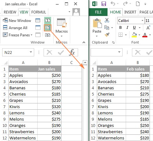
Imagine you have sales reports for two different periods and want to compare them directly. The “View Side by Side” feature can help you see which products performed better in each period.

To use this feature:

1. Open the two Excel workbooks you want to compare.
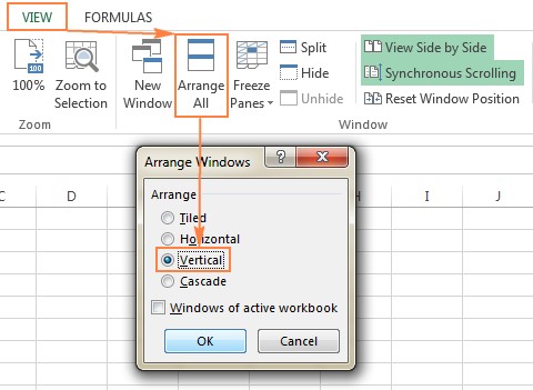
2. Go to the “View” tab, in the “Window” group, and click the “View Side by Side” button.

By default, the windows are displayed horizontally. To arrange them vertically, click the “Arrange All” button and select “Vertical.”

To scroll through both worksheets simultaneously, make sure the “Synchronous Scrolling” option is enabled. It’s located on the “View” tab, in the “Window” group, and is usually enabled automatically when you activate “View Side by Side” mode.

1.2 Arranging Multiple Excel Windows Side by Side

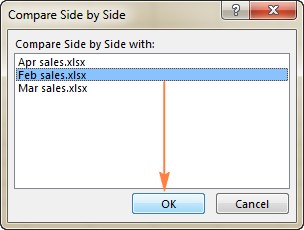
You can also view more than two Excel files at once. Open all the workbooks you want to compare, then click the “View Side by Side” button. A dialog box will appear, allowing you to select which files to display alongside the active workbook.

To view all open Excel files simultaneously, click the “Arrange All” button on the “View” tab, in the “Window” group, and choose your preferred arrangement: tiled, horizontal, vertical, or cascade.

1.3 Comparing Two Sheets in the Same Workbook

Sometimes the two sheets you want to compare are in the same workbook. To view them side by side:

1. Open the Excel file and go to the “View” tab, then the “Window” group, and click the “New Window” button.
2. This opens the same Excel file in a separate window.
3. Enable “View Side by Side” mode.
4. Select the first sheet in one window and the second sheet in the other window.

2. Using Formulas to Compare Two Excel Sheets for Differences

This method lets you identify cells with different values and create a difference report in a new worksheet.

To compare two Excel worksheets for differences:

1. Open a new, empty sheet.
2. Enter the following formula in cell A1:
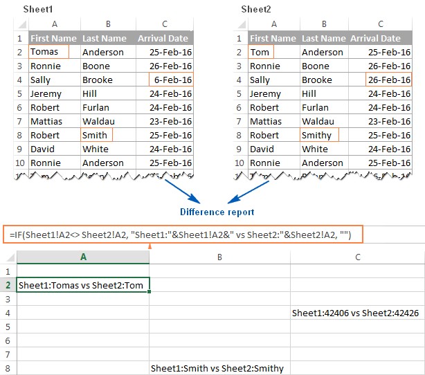
   =IF(Sheet1!A1<>Sheet2!A1, "Sheet1:"&Sheet1!A1&" vs Sheet2:"&Sheet2!A1, "")
3. Copy the formula down and to the right using the fill handle.

Due to the use of relative cell references, the formula will adjust based on its position, comparing corresponding cells in Sheet1 and Sheet2. The result will look like this:

This formula identifies cells with different values and displays the differences. However, it may not be ideal for dates, as they are presented as serial numbers.

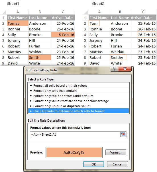
3. Highlighting Differences Between Two Sheets with Conditional Formatting

To highlight cells with different values using color, use Excel’s conditional formatting feature:

1. In the worksheet where you want to highlight differences, select all used cells by clicking the upper-left cell (usually A1) and pressing Ctrl+Shift+End.
2. On the “Home” tab, in the “Styles” group, click “Conditional Formatting” > “New Rule”.
3. Create a rule with the following formula: =A1<>Sheet2!A1
   (Replace Sheet2 with the name of the other sheet you are comparing).

This will highlight cells with different values in the color you choose.

4. Limitations of Built-in Excel Comparison Methods

While formulas and conditional formatting are useful, they have limitations:

• They only find differences in values and cannot compare formulas or cell formatting.
• They cannot identify added or deleted rows and columns. Adding or deleting a row/column will mark subsequent rows/columns as different.
• They work on a sheet level but cannot detect workbook-level structural differences like added or deleted sheets.

5. How to Compare Two Excel Sheets and Combine Unique Data Using the FILTER Function

The FILTER function is a powerful tool in Excel that allows you to extract data from a range based on specified criteria. When comparing two Excel sheets and combining unique data, FILTER can be incredibly useful for isolating the unique entries in each sheet and then combining them.

5.1 Understanding the FILTER Function

The basic syntax of the FILTER function is as follows:

=FILTER(array, include, [if_empty])

• array: The range of cells you want to filter.
• include: A logical array (an array of TRUE and FALSE values) that determines which rows or columns in the array to include in the result.
• [if_empty]: (Optional) The value to return if no entries meet the criteria.

5.2 Scenario: Combining Unique Customer Lists

Imagine you have two Excel sheets, each containing a list of customer names and email addresses. You want to create a single list that includes all customers but removes any duplicates. Here’s how you can use the FILTER function to achieve this:

Sheet 1: CustomerList1

Name	Email
John Doe	[email protected]
Jane Smith	[email protected]
Peter Jones	[email protected]

Sheet 2: CustomerList2

Name	Email
Jane Smith	[email protected]
Alice Brown	[email protected]
David Lee	[email protected]

5.3 Step-by-Step Guide to Combining Unique Data

1. Identify the Unique Values in Each Sheet:

   • First, determine which values are unique to CustomerList1. To do this, you’ll check if each name in CustomerList1 exists in CustomerList2.

2. Use the COUNTIF Function to Find Matches:

   • The COUNTIF function counts the number of cells within a range that meet a given criterion. You can use this to check if a name from CustomerList1 appears in CustomerList2.

3. Apply the FILTER Function to Extract Unique Values from CustomerList1:

   • Assuming your data in CustomerList1 is in columns A (Name) and B (Email), and in CustomerList2 it’s in columns D and E, use the following formula in a new sheet to extract the unique names and emails from CustomerList1:

   =FILTER(CustomerList1!A2:B4, ISERROR(MATCH(CustomerList1!A2:A4, CustomerList2!D2:D4, 0)))

   • Explanation:
     • CustomerList1!A2:B4 is the range containing the names and email addresses in the first list.
     • ISERROR(MATCH(CustomerList1!A2:A4, CustomerList2!D2:D4, 0)) checks if each name in CustomerList1 exists in CustomerList2. The MATCH function returns the position of the matched value, and ISERROR checks if MATCH returns an error (meaning the name is not found in CustomerList2).

4. Extract Unique Values from CustomerList2:

   • Similarly, use the FILTER function to extract unique values from CustomerList2:

   =FILTER(CustomerList2!D2:E4, ISERROR(MATCH(CustomerList2!D2:D4, CustomerList1!A2:A4, 0)))

   • Explanation:
     • CustomerList2!D2:E4 is the range containing the names and email addresses in the second list.
     • ISERROR(MATCH(CustomerList2!D2:D4, CustomerList1!A2:A4, 0)) checks if each name in CustomerList2 exists in CustomerList1.

5. Combine the Unique Lists:

   • Now that you have the unique values from both lists, you can combine them into a single list. Simply copy the results from the two FILTER formulas into a new table.

   • Combined Unique Customer List:

   Name	Email
   John Doe	[email protected]
   Peter Jones	[email protected]
   Alice Brown	[email protected]
   David Lee	[email protected]

5.4 Advantages of Using the FILTER Function

• Dynamic: The FILTER function provides a dynamic result. If you update the original customer lists, the filtered lists will automatically update.
• Efficient: It quickly extracts unique entries based on specified criteria, saving time and reducing manual errors.
• Readable: The formulas are relatively easy to understand, making them maintainable.

5.5 Considerations

• Data Structure: Ensure that your data is well-structured in both sheets. The FILTER function works best when the data is organized in a tabular format.
• Formula Adjustment: Adjust the cell ranges in the formulas to match the actual location of your data in the sheets.
• Error Handling: Include error handling (e.g., using IFERROR) to manage cases where the FILTER function might return errors.

By following these steps, you can efficiently compare two Excel sheets and combine unique data using the FILTER function. This method is particularly useful for managing customer lists, product inventories, and other data sets where maintaining unique and accurate records is essential.

6. Compare and Merge Copies of a Shared Workbook

Excel’s “Compare and Merge” feature is useful for merging different versions of the same Excel file, especially when multiple users collaborate on it. It allows you to view the changes and comments of all users at once.

To use this feature:

1. Share the Excel workbook before making it available to others. To share, click the “Share Workbook” button on the “Review” tab, in the “Changes” group, and select “Allow Changes by More Than One User…”.
2. Each user must save a copy of the shared workbook with a unique file name.

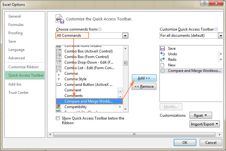
6.1 Enabling the Compare and Merge Workbooks Feature

The “Compare and Merge Workbooks” feature is available in Excel 2010 through Excel 365, but it’s not displayed by default. To add it to the Quick Access toolbar:

1. Open the Quick Access dropdown menu and select “More Commands.”
2. In the “Excel Options” dialog box, select “All Commands” under “Choose commands from.”
3. Scroll down to “Compare and Merge Workbooks”, select it, and click “Add”.
4. Click “OK”.

6.2 Comparing and Merging Workbooks

1. Open the primary version of the shared workbook.
2. Click the “Compare and Merge Workbooks” command on the Quick Access toolbar.
3. Select the copies of the shared workbook you want to merge and click “OK”.

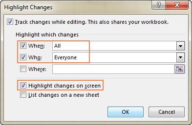
6.3 Reviewing the Changes

To see all the edits by different users:

1. Go to the “Review” tab > “Changes” group, and click “Track Changes” > “Highlight Changes”.
2. In the “Highlight Changes” dialog, select “All” in the “When” box, “Everyone” in the “Who” box, clear the “Where” box, select “Highlight changes on screen”, and click “OK”.

Excel highlights the column letters and row numbers in dark red to indicate rows and columns with differences. Edits from different users are marked with different colors. Hover over a cell to see who made the change.

The “Compare and Merge Workbooks” feature is only for copies of the same shared workbook, not different Excel files.

7. Third-Party Tools to Compare Excel Files

Built-in Excel options might not be sufficient for a comprehensive comparison of Excel sheets and workbooks. Third-party tools are designed specifically for comparing, updating, and merging Excel sheets and workbooks.

7.1 Synkronizer Excel Compare: Compare, Merge, and Update

The Synkronizer Excel Compare add-in can quickly compare, merge, and update two Excel files.

Key features include:

• Identifying differences between Excel sheets.
• Combining multiple Excel files into a single version.
• Highlighting differences.
• Showing relevant differences.
• Merging and updating sheets.
• Detailed difference reports.

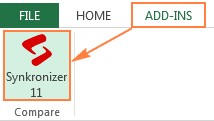
7.1.1 Comparing Two Excel Files for Differences

To run Synkronizer Excel Compare, go to the “Add-ins” tab and click the Synchronizer 11 icon.

1. Select the two workbooks to compare.
2. Select the sheets to compare. Synkronizer can automatically match sheets with the same names.
3. Choose a comparison option: compare as normal worksheets, compare with link options, compare as a database, or compare selected ranges.
4. Choose the content types to be compared (values, formulas, comments, formats, etc.).
5. Click the “Start” button.

7.1.2 Visualizing and Analyzing the Differences

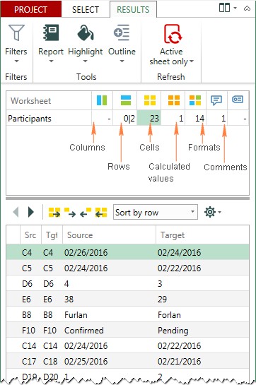
Synkronizer provides summary and detailed reports. The summary report shows all difference types, while the detailed report shows specific differences.

Clicking on a difference in the detailed report selects the corresponding cells on both sheets. You can also create a difference report in a separate workbook, either standard or hyperlinked.

7.1.3 Highlighting Differences Between Sheets

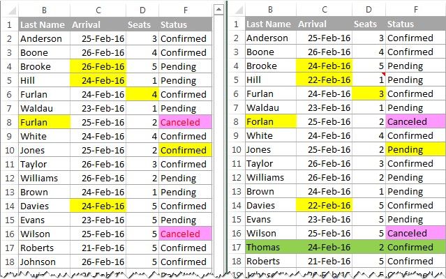
Synkronizer highlights differences by default: yellow for cell values, lilac for cell formats, and green for inserted rows. You can customize the highlighting by clicking the “Outline” button.

7.1.4 Update and Merge Sheets

The merge function allows you to transfer individual cells or move columns/rows from the source to the target sheet. Select the differences and click one of the update buttons to transfer the data.

7.2 Ablebits Compare Sheets for Excel

The Ultimate Suite includes Compare Sheets, a tool to compare worksheets in Excel.

The add-in features:

• A step-by-step wizard.
• Different comparison algorithms.
• A “Review Differences” mode.

1. Click the “Compare Sheets” button on the “Ablebits Data” tab, in the “Merge” group.
2. Select the two worksheets to compare.
3. Select the comparison algorithm: no key columns, by key columns, or cell-by-cell.
4. Specify which differences to highlight and how to mark them.
5. Click the “Compare” button.

7.2.1 Review and Merge Differences

The worksheets open side-by-side in “Review Differences” mode, with the first difference selected. Differences are highlighted with colors: blue for rows only in the first sheet, red for rows only in the second sheet, and green for different cells.

Use the toolbar to go through the differences and decide whether to merge or ignore them.

7.3 xlCompare: Compare and Merge Workbooks, Sheets, and VBA Projects

The xlCompare utility compares Excel files, worksheets, names, and VBA Projects. It identifies added, deleted, and changed data and allows you to quickly merge differences.

Other options include:

• Finding and removing duplicate records.
• Updating existing records with values from another sheet.
• Adding unique rows and columns.
• Merging updated records.
• Sorting data.
• Filtering comparison results.
• Highlighting comparison results.

7.4 Change pro for Excel: Compare Excel Sheets on Desktop and Mobile Devices

With Change pro for Excel, you can compare sheets on desktop and mobile devices.

Key features include:

• Finding differences in formulas and values.
• Identifying layout changes (added/deleted rows and columns).
• Recognizing embedded objects (charts, graphs, and images).
• Creating and printing difference reports.
• Filtering, sorting, and searching the difference report.
• Comparing files from Outlook or document management systems.
• Supporting all languages.

8. Online Services to Compare Excel Files

Online services allow you to compare Excel sheets for differences without installing any software. These services may not be ideal for sensitive information but can provide quick results.

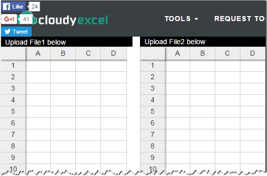
Services like XLComparator and CloudyExcel allow you to upload two Excel workbooks and highlight the differences in active sheets.

9. Utilizing Power Query for Advanced Data Combination

Power Query, available in Excel, provides advanced capabilities for data transformation and combination. This tool allows you to import data from multiple sources, clean it, and combine it based on specific criteria.

9.1 Importing Data into Power Query

1. Open Excel: Launch Microsoft Excel.

2. Go to the Data Tab: Click on the “Data” tab in the Excel ribbon.

3. Get Data: In the “Get & Transform Data” group, click on “Get Data.”

   • From File: Select “From File” and then choose “From Excel Workbook.”
   • Browse and Select: Browse to the location of your Excel file, select it, and click “Import.”
   • Navigator Window: The Navigator window will appear, showing the sheets and tables in your workbook. Select the sheet or table you want to import and click “Transform Data.” This opens the Power Query Editor.

9.2 Combining Tables in Power Query

1. Open Power Query Editor: Follow the steps in the previous section to open both tables in the Power Query Editor.

2. Append Queries:

   • Go to the “Home” tab in the Power Query Editor.

   • Click on “Append Queries” in the “Combine” group.

   • Select “Append Queries as New” to create a new query that combines the tables.

   • In the “Append” dialog box, select “Two tables” or “Three or more tables” depending on your scenario.

   • Add the tables you want to combine and click “OK.”

3. Remove Duplicates:

   • Select the columns you want to use to identify duplicates.
   • Go to the “Home” tab, click on “Remove Rows,” and select “Remove Duplicates.”

9.3 Cleaning and Transforming Data

Power Query provides a variety of tools to clean and transform your data before combining it:

• Rename Columns: Double-click on a column header to rename it.
• Change Data Types: Click on the data type icon next to a column header to change the data type (e.g., text, number, date).
• Remove Columns: Select a column, right-click, and choose “Remove” to delete it.
• Filter Rows: Click on the filter icon in a column header to filter rows based on specific criteria.
• Add Conditional Columns: Go to the “Add Column” tab and select “Conditional Column” to create new columns based on conditions.

9.4 Example: Combining Sales Data from Two Excel Sheets

Let’s say you have two Excel sheets containing sales data, and you want to combine them into a single table.

Sheet 1: SalesData_January

Product	Sales
Product A	100
Product B	150
Product C	120

Sheet 2: SalesData_February

Product	Sales
Product A	110
Product B	160
Product D	90

1. Import Data: Import both SalesData_January and SalesData_February into the Power Query Editor.

2. Append Queries:

   • Click “Append Queries as New.”
   • Add both tables to the append operation and click “OK.”

3. Remove Duplicates (if necessary): If you want to remove duplicate entries based on the “Product” column:

   • Select the “Product” column.
   • Go to “Remove Rows” and click “Remove Duplicates.”

4. Load Data to Excel:

   • Click “Close & Load” to load the combined data into a new Excel sheet.

Combined Sales Data

Product	Sales
Product A	100
Product B	150
Product C	120
Product A	110
Product B	160
Product D	90

9.5 Advantages of Using Power Query

• Versatility: Power Query can handle various data sources and complex transformations.
• Automation: Transformations are recorded as steps, allowing you to refresh the data with a single click.
• Efficiency: Power Query is optimized for large datasets, making it faster than manual methods.
• No Coding Required: It provides a user-friendly interface, reducing the need for complex formulas or scripting.

9.6 Best Practices

• Name Your Queries: Give your queries descriptive names to keep your workflow organized.
• Use Comments: Add comments to explain complex transformation steps.
• Validate Data: Always validate the combined data to ensure accuracy and completeness.
• Incremental Loading: For large datasets, consider using incremental loading to update only the new or changed data.

By using Power Query, you can efficiently combine and transform data from multiple Excel sheets, automate repetitive tasks, and ensure data quality. This tool is particularly useful for data analysts, business intelligence professionals, and anyone who needs to work with large and complex datasets.

10. Frequently Asked Questions (FAQ)

1. How do I compare two Excel files without seeing them side by side?
   • Use formulas or conditional formatting to highlight differences or use third-party tools designed for Excel comparison.
2. Can I compare Excel files with different layouts?
   • Yes, third-party tools like Synkronizer and Ablebits Compare Sheets offer algorithms to compare files with different layouts.
3. Is there a way to compare only specific columns in two Excel sheets?
   • Yes, many third-party tools and even some built-in Excel features allow you to select specific columns for comparison.
4. How can I find duplicate rows in two Excel sheets?
   • Use the COUNTIF function to identify rows with matching values in both sheets. You can then use filtering or conditional formatting to highlight these duplicates.
5. What is the best way to compare large Excel files?
   • Third-party tools and Power Query are better suited for comparing large Excel files, as they are optimized for handling large datasets efficiently.
6. Can I compare Excel files stored in different locations (e.g., SharePoint, OneDrive)?
   • Yes, many third-party tools support accessing files from various cloud storage services.
7. How do I ensure that the comparison results are accurate?
   • Validate the comparison results by manually checking a subset of the data. Also, ensure that the comparison settings are appropriate for your data structure.
8. Is it possible to automate the Excel comparison process?
   • Yes, you can use VBA scripts or third-party automation tools to automate the Excel comparison process.
9. How can I merge data from two Excel sheets while avoiding duplicates?
   • Use Power Query or the FILTER function to extract unique values from each sheet and then combine them into a single list.
10. Are online Excel comparison services secure?
    • Exercise caution when using online services, especially if your files contain sensitive information. Choose reputable services with secure data handling practices.

Conclusion

Comparing two Excel sheets and merging unique data can be a complex task, but with the right tools and techniques, it can be done efficiently and accurately. Whether you choose to use built-in Excel features, third-party tools, or online services, COMPARE.EDU.VN offers valuable insights and resources to help you find the best solution for your needs.

Ready to make data comparison easier? Visit compare.edu.vn for comprehensive guides, tool reviews, and expert advice to make informed decisions. Contact us at 333 Comparison Plaza, Choice City, CA 90210, United States, or Whatsapp: +1 (626) 555-9090.