How to Compare Two Excel Columns for Differences

Comparing columns in Excel is a fundamental skill for anyone working with data. Whether you’re reconciling financial records, cleaning customer lists, or analyzing sales figures, identifying differences between columns is often a crucial step. Microsoft Excel provides a range of built-in tools and formulas to accomplish this, from simple conditional formatting to more advanced functions. This guide will explore various techniques to effectively compare two Excel columns for differences, helping you pinpoint discrepancies and ensure data accuracy.

Comparing Two Excel Columns Row-by-Row

A common scenario is comparing data on a row-by-row basis. This is particularly useful when you need to see if corresponding entries in two columns are the same or different. Excel’s IF function is perfectly suited for this task.

Method 1: Using the IF Function for Basic Comparison

The IF function allows you to perform a logical test and return different values based on whether the test is true or false. In the context of comparing two columns, we can use it to check if the values in corresponding cells of two columns are equal or not.

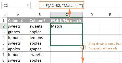
Formula for Identifying Matches

To find rows where the content of two cells in the same row is identical, for example, cells A2 and B2, you can use the following formula:

=IF(A2=B2,"Match","")

Enter this formula in a third column (say, column C) in the same row (C2). Then, drag the fill handle (the small square at the bottom-right of the cell C2) down to apply the formula to the rest of the rows. As you drag, the formula will automatically adjust to compare subsequent rows (A3 and B3, A4 and B4, and so on).

This formula checks if the value in cell A2 is equal to the value in cell B2. If they are the same, it returns “Match”; otherwise, it returns an empty string (“”).

Formula for Identifying Differences

Conversely, to highlight rows where the values in the two columns are different, simply change the equals sign (=) to the “not equal to” sign (<>):

=IF(A2<>B2,"Difference","")

This formula will return “Difference” if the values in A2 and B2 are not the same, and an empty string if they are identical.

Formula for Showing Both Matches and Differences

You can also modify the IF formula to display distinct messages for both matches and differences:

=IF(A2=B2,"Match","Difference")

Or:

=IF(A2<>B2,"Difference","Match")

The output will then clearly indicate whether each row contains matching or different values in the compared columns.

The IF function works seamlessly with numbers, dates, times, and text strings, making it a versatile tool for various data types.

Tip: For more advanced filtering based on row-by-row comparison, consider using Excel’s Advanced Filter. It allows for complex criteria to filter matches and differences between columns.

Method 2: Case-Sensitive Comparison with EXACT Function

By default, Excel’s comparison formulas are not case-sensitive, meaning “Apple” and “apple” are considered the same. If you need to perform a case-sensitive comparison, the EXACT function is the solution.

Formula for Case-Sensitive Matches

The EXACT function checks if two text strings are exactly the same, including case. Combined with the IF function, it can be used to find case-sensitive matches:

=IF(EXACT(A2, B2), "Match", "")

This formula returns “Match” only if A2 and B2 are identical in both value and case.

Formula for Case-Sensitive Differences

To identify case-sensitive differences, you can modify the formula to display a different output for mismatches:

=IF(EXACT(A2, B2), "Match", "Case Difference")

This will show “Case Difference” when the text is similar but the case is different, or if the text values themselves are different.

Comparing Multiple Columns in the Same Row

Excel also allows you to compare more than two columns within the same row. Here are a couple of scenarios and formulas for comparing multiple columns.

Scenario 1: Finding Matches Across All Cells in a Row

If you have several columns and need to identify rows where all cells in those columns have the same value, you can use the AND function in combination with IF.

Formula using AND for Multiple Column Match

For example, to check if cells A2, B2, and C2 all contain the same value, use:

=IF(AND(A2=B2, A2=C2), "Full Match", "")

This formula checks if A2 equals B2 AND A2 equals C2. If both conditions are true, it returns “Full Match”.

Formula using COUNTIF for Multiple Column Match

For a more scalable solution, especially when comparing many columns, the COUNTIF function is more efficient:

=IF(COUNTIF($A2:$E2, $A2)=5, "Full Match", "")

Here, $A2:$E2 is the range of columns being compared in row 2, and 5 is the total number of columns in that range. The formula counts how many times the value in A2 appears within the range A2:E2. If it appears 5 times (meaning all cells in the range have the same value as A2), it returns “Full Match”.

Scenario 2: Finding Matches in Any Two Cells within a Row

Sometimes you might need to know if any two or more cells within a row have matching values. The OR function is useful here.

Formula using OR for Any Two-Cell Match

To check if at least two out of three columns (A, B, C) in a row have the same value, you can use:

=IF(OR(A2=B2, B2=C2, A2=C2), "Match", "")

This formula checks if A2=B2 OR B2=C2 OR A2=C2. If any of these conditions are true, it returns “Match”.

Formula using COUNTIF for Any Two-Cell Match (Scalable)

For a larger number of columns, using multiple COUNTIF functions can be more manageable than a long OR statement:

=IF(COUNTIF(B2:D2,A2)+COUNTIF(C2:D2,B2)+(C2=D2)=0,"Unique","Match")

This formula becomes more complex but is more efficient for many columns. It essentially checks for matches between pairs of columns within the row. If the total count of matches is zero, it means no two cells match, and it returns “Unique”; otherwise, it returns “Match”.

Comparing Two Entire Columns for Matches and Differences

Beyond row-by-row comparisons, you may need to compare two entire columns to find values that exist in one column but not the other.

Method 1: Using COUNTIF for Column-Wide Comparison

The COUNTIF function can be used to search for values from one column within another column, helping to identify differences.

Formula to Find Values in Column A Not Present in Column B

To find values in column A that are not present in column B, use this formula in a new column (e.g., column C):

=IF(COUNTIF($B:$B, $A2)=0, "Not in Column B", "")

This formula counts how many times the value in cell A2 appears in the entire column B ($B:$B). If the count is 0 (meaning the value from A2 is not found in column B), it returns “Not in Column B”.

Tip: For very large datasets, instead of referencing the entire column ($B:$B), specifying a range (like $B$2:$B$1000) can improve performance.

Alternative Formulas using MATCH and ISERROR or Array Formulas

You can achieve the same result using MATCH and ISERROR functions:

=IF(ISERROR(MATCH($A2,$B$2:$B$10,0)),"Not in Column B","")

Or, with an array formula (remember to press Ctrl + Shift + Enter):

=IF(SUM(--($B$2:$B$10=$A2))=0, "Not in Column B", "")

These formulas also check if a value from column A exists in column B. If not, they indicate “Not in Column B”.

Identifying Both Matches and Differences

To identify both matches and differences in one formula, modify the IF and COUNTIF formula to display a different message for matches:

=IF(COUNTIF($B:$B, $A2)=0, "Not in Column B", "Found in Column B")

This will clearly label each value in column A as either “Found in Column B” or “Not in Column B”.

Pulling Matching Data from Two Lists

Sometimes, the goal is not just to identify differences but also to retrieve related data when a match is found between two columns (often in different tables or lists). Excel’s lookup functions are designed for this.

Using VLOOKUP, INDEX/MATCH, and XLOOKUP

Excel offers several powerful lookup functions, including VLOOKUP, INDEX/MATCH, and XLOOKUP (for Excel 2021 and Microsoft 365 users). These functions can compare values and, upon finding a match, return corresponding data from another column.

Example using Lookup Functions

Suppose you have product names in column D and want to compare them against product names in column A. If a match is found, you want to pull the sales figure from column B (corresponding to the matched product in column A).

VLOOKUP Formula:
=VLOOKUP(D2, $A$2:$B$6, 2, FALSE)
INDEX/MATCH Formula:
=INDEX($B$2:$B$6, MATCH($D2, $A$2:$A$6, 0))
XLOOKUP Formula (Excel 2021/365):
=XLOOKUP(D2, $A$2:$A$6, $B$2:$B$6)

These formulas search for the value in D2 within the range A2:A6. If a match is found, they return the value from the 2nd column of the lookup range (for VLOOKUP and INDEX/MATCH) or from the specified return range (for XLOOKUP). If no match is found, they typically return a #N/A error.

For a deeper dive into using VLOOKUP for comparing columns, refer to guides specifically on How to compare two columns using VLOOKUP.

Formula-Free Solution: Merge Tables Wizard

For users who prefer a more visual and intuitive approach, add-ins like the Merge Tables Wizard can simplify the process of comparing and merging data without writing formulas.

Highlighting Matches and Differences Visually

Conditional formatting is a powerful Excel feature to visually highlight cells based on specific criteria. This is ideal for quickly spotting matches and differences between columns.

Highlighting Matches and Differences Row-by-Row

Highlighting Matches in Each Row

To highlight cells in column A that have identical values in column B in the same row:

Select the range in column A you want to format.
Go to Home > Conditional Formatting > New Rule > Use a formula to determine which cells to format.
Enter the formula: =$B2=$A2 (assuming row 2 is the first data row). Ensure you use a relative row reference for column B (no $ before the row number).
Choose a formatting style (e.g., fill color) and click OK.

Highlighting Differences in Each Row

To highlight differences between column A and column B, use a similar process but with the formula:

=$B2<>$A2

For detailed steps on using formula-based conditional formatting, see How to create a formula-based conditional formatting rule.

Highlighting Unique Entries in Each List

When comparing two lists, you can highlight unique items (present in only one list) and duplicates (present in both).

Highlighting Unique Values in List 1 (Column A)

To highlight values in column A that are not found in column C (List 2):

Select the range in column A.
Create a new conditional formatting rule with the formula: =COUNTIF($C$2:$C$5, $A2)=0 (adjust range $C$2:$C$5 to your List 2 range).

Highlighting Unique Values in List 2 (Column C)

Similarly, to highlight unique values in column C (not in column A):

Select the range in column C.
Create a rule with the formula: =COUNTIF($A$2:$A$6, $C2)=0 (adjust range $A$2:$A$6 to your List 1 range).

Highlighting Matches (Duplicates) Between Two Columns

To highlight items that are present in both columns (duplicates or matches):

Highlighting Matches in List 1 (Column A)

Select the range in column A.
Use conditional formatting with the formula: =COUNTIF($C$2:$C$5, $A2)>0

Highlighting Matches in List 2 (Column C)

Select the range in column C.
Use conditional formatting with the formula: =COUNTIF($A$2:$A$6, $C2)>0

Highlighting Row Differences and Matches in Multiple Columns

When comparing multiple columns row-by-row, conditional formatting and Excel’s “Go To Special” feature offer quick visualization of matches and differences.

Highlighting Row Matches Across Multiple Columns

To highlight rows where all columns have identical values:

Select the rows you want to format.
Create a conditional formatting rule with one of these formulas:
- =AND($A2=$B2, $A2=$C2) (for 3 columns)
- =COUNTIF($A2:$C2, $A2)=3 (scalable for more columns, adjust ‘3’ to the number of columns).

Highlighting Row Differences Across Multiple Columns Using “Go To Special”

For quickly highlighting cells with different values within each row:

Select the range of columns you want to compare.
Go to Home > Find & Select > Go To Special.
Choose “Row differences” and click OK.
Excel will select cells that are different from the comparison cell in each row (the active cell in the selection).
Apply a fill color to the selected cells to highlight the differences.

Comparing Two Individual Cells

Comparing two individual cells is a simplified version of row-by-row column comparison. You can directly use the IF formulas mentioned earlier.

Formulas for Comparing Two Cells

To compare cell A1 and C1:

For Matches: =IF(A1=C1, "Match", "")
For Differences: =IF(A1<>C1, "Difference", "")

For more ways to compare individual cells, explore resources on comparing cells in Excel.

Formula-Free Column Comparison with Add-ins

For users seeking a solution without formulas or conditional formatting, specialized Excel add-ins like Compare Two Tables, part of Ultimate Suite, offer a user-friendly interface for comparing lists and tables.

Using Compare Two Tables Add-in

This add-in allows you to compare two lists or tables by selecting them directly, choosing the type of comparison (duplicates or unique values), and specifying columns for comparison. It provides options to highlight differences, identify matches in a status column, and more.

Steps to Compare Lists Using the Add-in

Open the Compare Tables tool from the Ablebits Data tab in Excel.
Select your first list (Table 1).
Select your second list (Table 2).
Choose to find “Duplicate values” (matches) or “Unique values” (differences).
Select the columns to compare from each list.
Choose an output option, such as “Highlight with color” or “Identify in the Status column”.

This add-in simplifies complex comparisons and provides a quick, visual way to analyze differences and matches in your Excel data.

Tip: When comparing lists in different worksheets or workbooks, using Excel’s view sheets side by side feature can be helpful for visual reference.

By mastering these techniques, you can efficiently compare columns in Excel for differences, ensuring data accuracy and gaining valuable insights from your spreadsheets.

Downloads

Compare Excel Lists – examples (.xlsx file)
Ultimate Suite – trial version (.exe file)