Comparing data across multiple Excel sheets can be challenging, but COMPARE.EDU.VN offers solutions to streamline this process. This article explores effective methods for comparing two different sheets in Excel, ensuring data accuracy and saving you time. Discover the best comparison strategies and data analysis techniques.
1. Understanding the Need for Sheet Comparison in Excel
Comparing two different sheets in Excel is a common task in data analysis and management. It’s crucial for identifying discrepancies, validating data integrity, and merging information from multiple sources. Whether you’re reconciling financial statements, tracking inventory, or analyzing survey results, the ability to compare sheets efficiently is essential.
- Data Validation: Ensuring data consistency across different sheets.
- Discrepancy Identification: Spotting differences and errors in data.
- Merging Information: Combining relevant data from multiple sheets.
- Trend Analysis: Comparing data over time to identify trends.
- Reporting: Creating comprehensive reports by consolidating data.
2. Basic Techniques for Comparing Excel Sheets
Several basic techniques can be used to compare two sheets in Excel, depending on the complexity of your data and the level of detail required.
- Manual Comparison: Visually inspecting sheets side-by-side.
- Sorting and Filtering: Arranging data to highlight differences.
- Conditional Formatting: Using color-coding to identify matches and mismatches.
- Simple Formulas: Employing basic formulas like
=IF()to compare cell values.
While these methods are straightforward, they can be time-consuming and prone to errors when dealing with large datasets. For more complex comparisons, more advanced techniques are necessary.
3. Using the IF Function for Cell-by-Cell Comparison
The IF function is a fundamental tool for comparing cell values in Excel. It allows you to specify a condition and return different results based on whether the condition is true or false.
- Syntax:
=IF(logical_test, value_if_true, value_if_false) - Example:
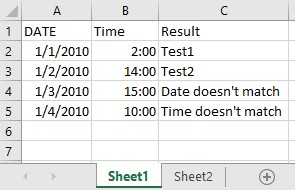
=IF(Sheet1!A1=Sheet2!A1, "Match", "Mismatch")
This formula compares the value in cell A1 of Sheet1 with the value in cell A1 of Sheet2. If the values are identical, it returns “Match”; otherwise, it returns “Mismatch”.
Advantages:
- Simple and easy to understand.
- Can be customized to compare different data types.
- Useful for highlighting specific differences.
Disadvantages:
- Time-consuming for large datasets.
- Requires manual entry of formulas for each cell.
- Not suitable for complex comparisons involving multiple criteria.
4. Leveraging Conditional Formatting for Visual Comparison
Conditional formatting is a powerful feature in Excel that allows you to automatically apply formatting to cells based on their values or formulas. This can be used to visually highlight differences between two sheets.
- Highlighting Duplicate Values: Identifying cells with identical values in both sheets.
- Highlighting Unique Values: Spotting cells with different values in each sheet.
- Using Color Scales: Applying a gradient of colors to represent the magnitude of differences.
Steps to Use Conditional Formatting:
- Select the range of cells you want to compare in Sheet1.
- Go to “Home” > “Conditional Formatting” > “New Rule.”
- Choose “Use a formula to determine which cells to format.”
- Enter a formula that compares the selected cells with the corresponding cells in Sheet2.
- Specify the formatting you want to apply (e.g., background color, font style).
Example Formula:
- To highlight differences:
=Sheet1!A1<>Sheet2!A1 - To highlight matches:
=Sheet1!A1=Sheet2!A1
5. Employing the VLOOKUP Function for Data Matching
The VLOOKUP function is used to search for a value in one sheet and return a corresponding value from another sheet. This is particularly useful when you have a common identifier in both sheets, such as an ID number or product code.
- Syntax:
=VLOOKUP(lookup_value, table_array, col_index_num, [range_lookup]) lookup_value: The value you want to search for.table_array: The range of cells containing the data you want to search in (including the column with the return value).col_index_num: The column number in thetable_arraythat contains the return value.[range_lookup]: Optional.TRUEfor approximate match,FALSEfor exact match.
Example:
Suppose you have a list of product IDs in Sheet1 and corresponding prices in Sheet2. To retrieve the price of a product from Sheet2 and display it in Sheet1, you can use the following formula in Sheet1:
=VLOOKUP(A2, Sheet2!A:B, 2, FALSE)Here, A2 is the product ID in Sheet1, Sheet2!A:B is the range containing the product IDs and prices in Sheet2, 2 is the column number with the prices, and FALSE ensures an exact match.
6. Using the MATCH and INDEX Functions for Flexible Lookup
While VLOOKUP is useful, it has limitations. For example, it can only look up values in the leftmost column of the table array. The MATCH and INDEX functions provide a more flexible alternative.
MATCHFunction: Returns the position of a value in a range.- Syntax:
=MATCH(lookup_value, lookup_array, [match_type])
- Syntax:
INDEXFunction: Returns the value at a specific position in a range.- Syntax:
=INDEX(array, row_num, [column_num])
- Syntax:
Combining MATCH and INDEX:
=INDEX(Sheet2!B:B, MATCH(A2, Sheet2!A:A, 0))This formula searches for the value in cell A2 of Sheet1 in column A of Sheet2 using MATCH. It then uses INDEX to return the corresponding value from column B of Sheet2.
7. Comparing Entire Columns or Rows Using Array Formulas
Array formulas allow you to perform calculations on entire arrays (ranges of cells) at once. This can be used to compare entire columns or rows between two sheets.
-
Entering Array Formulas: Press
Ctrl + Shift + Enterafter typing the formula. Excel will automatically add curly braces{}around the formula. -
Example: To compare column A of Sheet1 with column A of Sheet2 and return
TRUEif they are identical orFALSEif they are not:=Sheet1!A1:A10=Sheet2!A1:A10
After entering this formula as an array formula, Excel will return an array of TRUE and FALSE values, indicating whether each corresponding cell in the two columns is identical.
8. Utilizing the SUMPRODUCT Function for Counting Matches
The SUMPRODUCT function multiplies corresponding components in given arrays and returns the sum of those products. This can be used to count the number of matches between two sheets.
-
Syntax:
=SUMPRODUCT((array1=array2)*(array3=array4)) -
Example: To count the number of rows where both column A and column B match between Sheet1 and Sheet2:
=SUMPRODUCT((Sheet1!A1:A100=Sheet2!A1:A100)*(Sheet1!B1:B100=Sheet2!B1:B100))
This formula compares the values in columns A and B of Sheet1 with the corresponding values in Sheet2. It multiplies the results, so only rows where both columns match will contribute to the sum.
9. Employing Excel’s Built-in “Compare Side by Side” Feature
Excel offers a built-in feature that allows you to view and compare two sheets side by side. This can be useful for visually inspecting differences and scrolling through the data simultaneously.
- Steps to Use “Compare Side by Side”:
- Open both Excel sheets you want to compare.
- Go to the “View” tab.
- Click on “View Side by Side” in the “Window” group.
- If you have more than two sheets open, Excel will prompt you to select the second sheet.
- Enable “Synchronous Scrolling” to scroll both sheets simultaneously.
This feature is particularly helpful for identifying patterns and trends that might be missed when comparing sheets individually.
10. Using Power Query for Advanced Data Comparison and Transformation
Power Query is a powerful data transformation and preparation tool built into Excel. It allows you to import data from various sources, clean and transform it, and load it into Excel for analysis. Power Query can be used to compare two sheets, identify differences, and merge data.
* **Importing Data:** Load data from both sheets into Power Query.
* **Merging Queries:** Combine the data from both sheets based on a common identifier.
* **Identifying Differences:** Use Power Query's transformation capabilities to identify and highlight differences between the two datasets.
* **Loading Results:** Load the transformed data back into Excel for further analysis.
Example:
Let’s say you have two sheets with customer data. Sheet1 contains the most up-to-date information, while Sheet2 is an older version. You want to identify customers who have new addresses in Sheet1 compared to Sheet2.
- Import Data: Load both Sheet1 and Sheet2 into Power Query using “Data” > “Get & Transform Data” > “From Table/Range”.
- Merge Queries:
- In Power Query Editor, select Sheet1 query.
- Go to “Home” > “Merge Queries”.
- Select Sheet2 query to merge with.
- Choose the common identifier column (e.g., Customer ID) for merging.
- Select the “Left Outer” join kind to keep all rows from Sheet1 and matching rows from Sheet2.
- Expand Merged Column:
- Expand the merged column to bring in relevant columns from Sheet2 (e.g., Old Address).
- Compare Addresses:
- Add a conditional column to compare the new address (from Sheet1) with the old address (from Sheet2). Use “Add Column” > “Conditional Column”.
- Set the condition to check if New Address is not equal to Old Address.
- If true, mark it as “Address Changed”; otherwise, mark it as “No Change”.
- Load Results: Load the transformed data back into Excel using “Home” > “Close & Load”.
Now, you have a table in Excel showing customers with changed addresses.
11. Creating Custom Functions with VBA for Specialized Comparisons
For highly specialized comparisons, you can create custom functions using Visual Basic for Applications (VBA). VBA allows you to write code that extends Excel’s functionality and performs complex tasks.
- Accessing VBA Editor: Press
Alt + F11to open the VBA editor. - Inserting a Module: Go to “Insert” > “Module.”
- Writing a Custom Function: Define a function that takes input values from the sheets you want to compare and returns a result based on your specific comparison criteria.
Example:
Here’s an example of a VBA function that compares two ranges and returns the number of differences:
Function CompareRanges(Range1 As Range, Range2 As Range) As Long
    Dim i As Long, j As Long
    Dim diffCount As Long

    diffCount = 0

    For i = 1 To Range1.Rows.Count
        For j = 1 To Range1.Columns.Count
            If Range1.Cells(i, j).Value <> Range2.Cells(i, j).Value Then
                diffCount = diffCount + 1
            End If
        Next j
    Next i

    CompareRanges = diffCount
End Function
To use this function in Excel, you would enter a formula like:
=CompareRanges(Sheet1!A1:C10, Sheet2!A1:C10)This will return the number of cells that are different between the two ranges.
12. Third-Party Excel Add-ins for Advanced Comparison
Several third-party Excel add-ins are available that provide advanced comparison features beyond what Excel offers natively. These add-ins often include features such as:
- Detailed difference reports: Highlighting specific differences between sheets.
- Automated comparison: Automatically comparing sheets based on predefined criteria.
- Data synchronization: Synchronizing data between sheets to ensure consistency.
- Version control: Tracking changes to sheets over time.
Some popular Excel add-ins for comparison include:
- Spreadsheet Compare: A Microsoft tool that is part of Office Professional Plus.
- Beyond Compare: A powerful comparison tool for files, folders, and spreadsheets.
- XL Comparator: An Excel add-in specifically designed for comparing spreadsheets.
13. Strategies for Handling Large Datasets
Comparing large datasets in Excel can be challenging due to performance limitations. Here are some strategies for handling large datasets effectively:
- Use Efficient Formulas: Opt for formulas that are optimized for performance, such as
INDEXandMATCHinstead ofVLOOKUP. - Disable Automatic Calculations: Turn off automatic calculations while performing comparisons to improve performance.
- Use Excel Tables: Convert your data ranges into Excel tables, which are optimized for performance and can handle large datasets more efficiently.
- Split Data into Smaller Chunks: Divide your data into smaller, more manageable chunks and compare them separately.
- Use Power Query: Power Query is designed to handle large datasets efficiently and can perform complex transformations without slowing down Excel.
14. Best Practices for Ensuring Accurate Comparisons
To ensure accurate comparisons between two sheets in Excel, it’s essential to follow best practices:
- Verify Data Types: Ensure that the data types in the columns you are comparing are consistent (e.g., numbers should be formatted as numbers, dates should be formatted as dates).
- Handle Missing Values: Decide how you want to handle missing values (e.g., treat them as zero, ignore them, or replace them with a specific value).
- Trim Whitespace: Remove any leading or trailing whitespace from your data, as this can cause comparisons to fail.
- Use Consistent Formatting: Apply consistent formatting to your data to ensure that comparisons are accurate.
- Test Your Formulas: Before applying your formulas to your entire dataset, test them on a small sample to ensure that they are working correctly.
15. Common Mistakes to Avoid When Comparing Sheets
Several common mistakes can lead to inaccurate comparisons between two sheets in Excel. Avoiding these mistakes can help you ensure the accuracy of your results:
- Incorrect Cell References: Double-check your cell references to ensure that you are comparing the correct cells.
- Mismatched Data Types: Ensure that the data types in the columns you are comparing are consistent.
- Ignoring Case Sensitivity: Be aware that Excel comparisons are case-insensitive by default. If you need to perform case-sensitive comparisons, use the
EXACTfunction. - Overlooking Hidden Rows or Columns: Hidden rows or columns can affect the results of your comparisons. Make sure to unhide them before performing your comparisons.
- Not Freezing Panes: When comparing large sheets, freeze panes to keep the header rows and columns visible while scrolling.
16. Real-World Examples of Comparing Excel Sheets
Here are some real-world examples of how comparing Excel sheets can be used in different industries and scenarios:
- Finance: Reconciling bank statements with internal records, comparing budget versus actual expenses.
- Inventory Management: Tracking inventory levels across different warehouses, comparing sales forecasts with actual sales.
- Human Resources: Comparing employee performance reviews, tracking employee demographics.
- Marketing: Analyzing campaign performance across different channels, comparing customer demographics with target market profiles.
- Research: Comparing survey results, analyzing experimental data.
17. Comparing Data Based on Multiple Criteria
Sometimes, you need to compare data based on multiple criteria. This can be achieved by combining multiple IF functions or using more complex formulas.
-
Combining
IFFunctions:=IF(AND(Sheet1!A1=Sheet2!A1, Sheet1!B1=Sheet2!B1), "Match", "Mismatch")This formula checks if both column A and column B match between Sheet1 and Sheet2.
-
Using
SUMPRODUCTwith Multiple Criteria:=SUMPRODUCT((Sheet1!A1:A100=Sheet2!A1:A100)*(Sheet1!B1:B100=Sheet2!B1:B100)*(Sheet1!C1:C100=Sheet2!C1:C100))This formula counts the number of rows where columns A, B, and C all match between Sheet1 and Sheet2.
18. Tips for Optimizing Your Comparison Workflow
To optimize your comparison workflow in Excel, consider the following tips:
- Plan Your Comparison: Before you start, clearly define what you want to compare and what criteria you will use.
- Organize Your Data: Ensure that your data is well-organized and consistent across both sheets.
- Use Named Ranges: Use named ranges to make your formulas easier to read and understand.
- Create Templates: Create templates for common comparison tasks to save time and ensure consistency.
- Document Your Process: Document your comparison process so that you can easily repeat it in the future and share it with others.
19. Using the EXACT Function for Case-Sensitive Comparisons
By default, Excel comparisons are case-insensitive. If you need to perform case-sensitive comparisons, use the EXACT function.
- Syntax:
=EXACT(text1, text2) - Example:
=EXACT(Sheet1!A1, Sheet2!A1)
This formula returns TRUE if the values in cell A1 of Sheet1 and Sheet2 are identical, including case, and FALSE otherwise.
20. Advanced Filtering Techniques for Targeted Comparison
Advanced filtering techniques can help you focus on specific subsets of your data, making comparisons more targeted and efficient.
- Using Advanced Filter: Use Excel’s Advanced Filter feature to extract specific records from one sheet based on criteria in another sheet.
- Filtering with Multiple Criteria: Use multiple criteria to filter your data and focus on specific subsets of records.
- Using Wildcard Characters: Use wildcard characters (e.g.,
*,?) to filter data based on partial matches.
21. Automating the Comparison Process with Macros
Macros can be used to automate the comparison process in Excel, saving you time and reducing the risk of errors.
- Recording Macros: Record a macro to automate a series of steps, such as formatting data, applying formulas, and filtering results.
- Writing VBA Code: Write VBA code to create custom macros that perform more complex comparison tasks.
- Assigning Macros to Buttons: Assign macros to buttons on your worksheet to make them easy to run.
22. Best Practices for Data Cleaning Before Comparison
Before comparing two sheets, it’s essential to clean your data to ensure accuracy. Here are some best practices for data cleaning:
- Remove Duplicate Records: Identify and remove duplicate records from your data.
- Correct Errors: Correct any errors in your data, such as spelling mistakes or incorrect values.
- Standardize Data: Standardize your data by converting it to a consistent format (e.g., converting all dates to the same format).
- Handle Missing Values: Decide how you want to handle missing values and apply a consistent approach.
23. The Role of Data Visualization in Comparison
Data visualization can play a crucial role in comparing two sheets by providing a visual representation of the differences.
- Charts: Use charts to compare data series, identify trends, and highlight differences.
- Sparklines: Use sparklines to display trends within a single cell.
- Conditional Formatting: Use conditional formatting to visually highlight differences between sheets.
24. Understanding Data Integrity and Consistency
Data integrity refers to the accuracy and consistency of data over its lifecycle. Maintaining data integrity is essential for ensuring that your comparisons are accurate and reliable.
- Data Validation: Use data validation rules to prevent users from entering invalid data.
- Regular Audits: Conduct regular audits of your data to identify and correct any errors.
- Version Control: Use version control to track changes to your data and ensure that you are always working with the most up-to-date version.
25. Exploring Advanced Excel Functions for Data Analysis
Excel offers a variety of advanced functions that can be used for data analysis and comparison.
AGGREGATE: Performs calculations on a range of cells, ignoring errors and hidden rows.FREQUENCY: Calculates the frequency distribution of a set of values.TRANSPOSE: Transposes a range of cells, converting rows to columns and vice versa.GETPIVOTDATA: Extracts data from a PivotTable.
26. Data Comparison for Financial Analysis
Comparing data in Excel is critical for financial analysis, ensuring accuracy and providing insights into financial performance.
- Budget vs. Actual Analysis: Compare budgeted figures against actual financial results to identify variances and assess performance.
- Trend Analysis: Analyze financial data over multiple periods to identify trends and patterns.
- Ratio Analysis: Calculate and compare financial ratios to assess profitability, liquidity, and solvency.
- Variance Analysis: Investigate and explain significant variances between budgeted and actual results.
27. How Data Comparison Aids in Project Management
Data comparison is instrumental in project management for tracking progress, managing resources, and ensuring projects stay on track.
- Task Comparison: Compare planned task durations against actual durations to identify delays and assess project progress.
- Resource Allocation: Compare planned resource allocation against actual resource usage to optimize resource management.
- Cost Tracking: Compare budgeted costs against actual costs to monitor project expenses and identify cost overruns.
- Milestone Tracking: Compare planned milestone completion dates against actual completion dates to track project milestones.
28. Using Excel for Scientific Data Comparison
Excel is frequently used in scientific research to compare and analyze experimental data, validate results, and draw conclusions.
- Statistical Analysis: Perform statistical tests to compare different datasets and determine if the differences are statistically significant.
- Data Visualization: Create charts and graphs to visualize scientific data and identify trends and patterns.
- Curve Fitting: Use Excel’s curve-fitting tools to model scientific data and compare different models.
- Error Analysis: Analyze errors in scientific data to assess the accuracy and reliability of the results.
29. Data Privacy and Security Considerations
When comparing sensitive data in Excel, it’s important to consider data privacy and security.
- Encryption: Encrypt your Excel files to protect them from unauthorized access.
- Password Protection: Password-protect your Excel files to prevent unauthorized users from opening or modifying them.
- Data Masking: Mask sensitive data to protect it from being viewed or copied.
- Access Controls: Implement access controls to restrict access to sensitive data.
30. FAQs About Comparing Two Different Sheets in Excel
Q1: What is the easiest way to compare two sheets in Excel?
A1: The easiest way to compare two sheets in Excel is to use conditional formatting to highlight differences.
Q2: Can I compare two sheets in Excel for differences automatically?
A2: Yes, you can use formulas like =IF() or VLOOKUP, or use Power Query, to automate the comparison process and identify differences.
Q3: How do I compare two columns in Excel for matches?
A3: Use the IF function to compare corresponding cells in the two columns and return a value indicating whether they match. For example, =IF(A1=B1, "Match", "Mismatch").
Q4: What is the best way to compare large datasets in Excel?
A4: For large datasets, use Power Query or optimized formulas like INDEX and MATCH. Disable automatic calculations and split the data into smaller chunks if necessary.
Q5: How can I compare two sheets and highlight the differences?
A5: Use conditional formatting with a formula that compares the cells and applies formatting to highlight the differences.
Q6: Is there a built-in feature in Excel to compare sheets side by side?
A6: Yes, Excel has a “View Side by Side” feature under the “View” tab that allows you to compare two sheets simultaneously.
Q7: How do I compare two Excel files for differences?
A7: You can use Excel’s “Compare Side by Side” feature or use third-party tools like Spreadsheet Compare (part of Office Professional Plus) to compare entire Excel files.
Q8: Can I perform a case-sensitive comparison in Excel?
A8: Yes, use the EXACT function to perform a case-sensitive comparison.
Q9: How do I count the number of matches between two sheets?
A9: Use the SUMPRODUCT function with a formula that compares the values in the two sheets and counts the number of matches.
Q10: What is Power Query, and how can it help with comparing sheets?
A10: Power Query is a data transformation tool in Excel that allows you to import, clean, and transform data. You can use it to merge data from two sheets, identify differences, and load the results back into Excel.
Comparing two different sheets in Excel can be a complex task, but with the right techniques and tools, it can be done efficiently and accurately. Whether you’re using basic formulas, conditional formatting, or advanced tools like Power Query and VBA, the key is to understand your data, plan your comparison, and follow best practices.
Ready to streamline your data comparison process and make informed decisions? Visit compare.edu.vn at 333 Comparison Plaza, Choice City, CA 90210, United States or contact us via Whatsapp at +1 (626) 555-9090 for more expert insights and comparison tools. Your path to smarter data analysis starts here. Navigate the complexities of data comparison with ease and confidence today.