Comparing data across two Excel sheets is a common task, whether you’re tracking changes, merging data, or identifying discrepancies. This article provides a comprehensive guide on various techniques for comparing columns in two Excel spreadsheets, ranging from simple visual inspection to leveraging powerful formulas and third-party tools.
Side-by-Side Comparison for Quick Checks
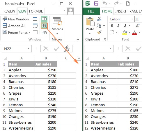
For smaller datasets and straightforward comparisons, viewing two Excel files side-by-side offers a quick visual solution.
- Open both Excel workbooks.
- Go to the View tab > Window group > click View Side by Side. This arranges the windows horizontally. For vertical arrangement, click Arrange All and choose Vertical.
- Enable Synchronous Scrolling (usually enabled by default in side-by-side mode). This allows simultaneous scrolling through both sheets, facilitating row-by-row comparison.
This method allows for a quick scan to identify obvious differences but is less effective for large datasets or subtle variations.
Comparing Values Using Formulas: Creating a Difference Report
Excel formulas provide a more precise method to pinpoint differences in values between two sheet columns.
- Open a new sheet for the difference report.
- In cell A1, enter the formula:
=IF(Sheet1!A1<>Sheet2!A1,"Sheet1: "&Sheet1!A1&" vs Sheet2: "&Sheet2!A1,""). This compares cell A1 in both sheets. If they differ, it displays both values; otherwise, it leaves the cell blank. - Drag the fill handle (the small square at the bottom right of the cell) down and across to apply the formula to the entire data range.
This formula-based approach creates a detailed report highlighting all value discrepancies. Note that dates might appear as serial numbers.
Highlighting Discrepancies with Conditional Formatting
Visualizing differences directly within the sheet is possible using conditional formatting.
- Select all cells in the sheet where you want to highlight differences.
- Go to Home tab > Styles group > Conditional Formatting > New Rule.
- Select “Use a formula to determine which cells to format”.
- Enter the formula:
=A1<>Sheet2!A1(adjusting “Sheet2” to the actual sheet name). - Choose a formatting style to highlight the differing cells.
This visually emphasizes the cells with differing values without creating a separate report.
Advanced Comparison Techniques: Third-Party Tools
While built-in Excel features offer basic comparison functionalities, dedicated tools provide more comprehensive solutions, particularly for complex comparisons involving formulas, formatting, and large datasets.
Several third-party tools offer advanced features:
- Synkronizer Excel Compare: Offers comparison, merging, and updating capabilities with detailed reports and highlighting.
- Ablebits Compare Sheets: Provides a user-friendly wizard, various comparison algorithms, and a review differences mode for efficient analysis and merging.
- xlCompare: Compares workbooks, sheets, and VBA projects, enabling merging, duplicate removal, and data updating.
These tools cater to more intricate comparison needs, offering features beyond the scope of built-in Excel functions.
Conclusion
Choosing the right method for comparing Excel sheet columns depends on the complexity and scale of your task. For quick visual checks, side-by-side viewing suffices. Formulas and conditional formatting offer more precise comparisons for moderate datasets. For complex scenarios involving large datasets, formulas, formatting, or merging requirements, dedicated third-party tools provide the most comprehensive solutions.