How to Compare Two Data Sets in Excel for Differences

Comparing two data sets in Excel is crucial for identifying discrepancies, duplicates, or missing information. Whether you’re reconciling financial records, validating customer databases, or tracking inventory changes, Excel provides powerful tools to streamline this process. This guide explores five effective methods to compare two data sets in Excel for differences, utilizing formulas, conditional formatting, and built-in features.

Comparing Data Sets in Excel: 5 Effective Methods

Efficiently comparing data in Excel allows for accurate analysis and informed decision-making. Let’s delve into five distinct methods for comparing two data sets:

1. Conditional Formatting for Visual Comparison

Conditional formatting highlights cells based on specific criteria, providing a visual representation of differences.

1. Select Data and Access Conditional Formatting: Select the data range encompassing both lists. Navigate to the “Home” tab and click “Conditional Formatting.”

2. Highlight Duplicate or Unique Values: Choose “Highlight Cells Rules” and select either “Duplicate Values” to highlight matching entries or “Unique Values” to emphasize discrepancies.

3. Customize Formatting: Select a formatting style from the dropdown menu to visually distinguish the highlighted cells. Click “OK” to apply the formatting.

.webp)

2. Cell-by-Cell Comparison with the Equal Sign Operator

This method compares individual cells and returns “TRUE” for matches and “FALSE” for mismatches.

1. Insert a New Column: Insert a new column adjacent to the two lists.

2. Apply Formula: In the first cell of the new column, enter the formula =A2=B2 (assuming your lists start in A2 and B2).

3. Drag Down Formula: Drag the fill handle down to apply the formula to all rows, generating a column of TRUE/FALSE values indicating matches and discrepancies.

.webp)

3. Identifying Matches and Missing Values with VLOOKUP

VLOOKUP searches for a value from the first list within the second list.

1. Enter Data and Select Result Column: Ensure your lists are entered into separate columns. Choose a third column for the results.

2. Apply VLOOKUP Formula: In the first cell of the results column, enter =VLOOKUP(A2,$B$2:$B$9,1,FALSE). Adjust the range $B$2:$B$9 to encompass your second list.

3. Interpret Results: Drag the formula down. Matching values will be displayed; “#N/A” indicates a value from the first list is missing in the second.

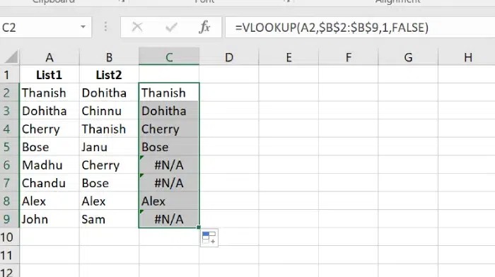Using VLOOKUP to find matches in Excel

4. Highlighting Row Differences

This method highlights entire rows where differences exist.

1. Select Data Range: Select the entire data range containing both lists.

2. Access “Go To Special”: Press F5 to open the “Go To Special” dialog box. Click “Special.”

3. Select “Row Differences”: Choose “Row differences” and click “OK.” Excel will highlight rows with any discrepancies.

.webp)

5. Using IF Condition for “Matching” or “Not Matching” Results

This method provides a clear text indication of matching or non-matching rows.

1. Enter Data: Input your lists into separate columns.

2. Apply IF Formula: In a new column, enter the formula =IF(A2=B2,"Matching","Not Matching").

3. Extend Formula: Drag the formula down to apply it to all rows, displaying “Matching” or “Not Matching” for each row comparison.

.webp)

Conclusion

Excel offers a versatile toolkit for comparing data sets. By mastering these five methods, you can efficiently identify differences, ensure data accuracy, and gain valuable insights from your data. Choose the technique that best suits your specific needs and data structure for effective data comparison and analysis.