How to Compare Two Columns to Find Matches in Excel

Discover How To Compare Two Columns To Find Matches In Excel using various techniques with COMPARE.EDU.VN, from simple formulas to advanced conditional formatting. Comparing two columns in Excel is a common need, and this guide provides detailed methods to identify matching data, highlight differences, and streamline your data analysis. Unlock the power of Excel data comparison, and enhance your spreadsheet skills with these easy-to-follow instructions.

1. Why Comparing Columns in Excel is Essential

Excel is a powerful tool for data management, analysis, and presentation. Data analysts and professionals across various fields rely on Excel to store, manipulate, and interpret information. The ability to compare two columns in Excel is a fundamental skill that can significantly improve efficiency and accuracy.

1.1. The Importance of Data Comparison

In many scenarios, you need to ensure data consistency, identify duplicates, or find missing values. Manually comparing columns in large spreadsheets can be time-consuming and prone to errors. Automating this process with Excel’s built-in features and formulas not only saves time but also reduces the risk of human error.

1.2. Use Cases for Column Comparison

Here are some common use cases where comparing two columns in Excel is invaluable:

Data Validation: Verifying that data entries in one column match corresponding entries in another column.
Duplicate Identification: Finding and removing duplicate entries in a dataset.
Missing Value Detection: Identifying values present in one column but missing in another.
Data Integration: Merging and synchronizing data from different sources.
Auditing: Ensuring compliance with data standards and regulations.

1.3. Challenges in Manual Comparison

Manual comparison becomes increasingly challenging as the size and complexity of the data grow. It’s easy to overlook subtle differences or miss entire entries, leading to inaccurate conclusions. Therefore, mastering automated comparison techniques in Excel is crucial for effective data analysis.

2. Basic Techniques for Comparing Two Columns

Excel offers several straightforward methods to compare two columns. These techniques are easy to implement and suitable for small to medium-sized datasets.

2.1. Using the Equals Operator (=)

The equals operator (=) is the simplest way to compare two columns on a row-by-row basis. This method returns TRUE if the values in the corresponding rows are identical and FALSE otherwise.

2.1.1. Step-by-Step Guide

Open your Excel spreadsheet: Ensure that the two columns you want to compare are visible.
Insert a new column: Create a new column next to the columns you are comparing (e.g., column C).
Enter the formula: In the first cell of the new column (e.g., C2), enter the formula =A2=B2.
Drag the formula down: Drag the fill handle (the small square at the bottom-right corner of the cell) down to apply the formula to all rows.

2.1.2. Interpreting the Results

The new column will display TRUE for rows where the values in columns A and B match and FALSE for rows where they differ. This method provides a quick visual indication of matching and non-matching entries.

2.2. Using the IF Function

The IF function allows you to display custom messages based on whether the values in two columns match or differ. This method provides more flexibility in presenting the comparison results.

2.2.1. Basic IF Function

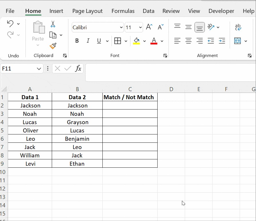
The basic syntax of the IF function for comparing two columns is =IF(A2=B2, "Match", "Not Match"). This formula checks if the value in cell A2 is equal to the value in cell B2. If they are equal, it displays “Match”; otherwise, it displays “Not Match”.

2.2.2. Step-by-Step Guide

Open your Excel spreadsheet: Ensure that the two columns you want to compare are visible.
Insert a new column: Create a new column next to the columns you are comparing (e.g., column C).
Enter the formula: In the first cell of the new column (e.g., C2), enter the formula =IF(A2=B2, "Match", "Not Match").
Drag the formula down: Drag the fill handle down to apply the formula to all rows.

2.2.3. Identifying Mismatches

To identify mismatches, you can modify the formula to =IF(A2<>B2, "Mismatch", "Match"). This formula checks if the value in cell A2 is not equal to the value in cell B2. If they are not equal, it displays “Mismatch”; otherwise, it displays “Match”.

2.3. Using the EXACT Function

The EXACT function is case-sensitive, meaning it considers uppercase and lowercase letters as different. This function is useful when you need to compare text strings that must match exactly.

2.3.1. Syntax of the EXACT Function

The syntax of the EXACT function is =EXACT(text1, text2). This function compares two text strings and returns TRUE if they are identical, including case, and FALSE otherwise.

2.3.2. Combining with the IF Function

To display custom messages, you can combine the EXACT function with the IF function: =IF(EXACT(A2, B2), "Match", "Not Match"). This formula checks if the text in cell A2 is exactly the same as the text in cell B2. If they are identical, it displays “Match”; otherwise, it displays “Not Match”.

2.3.3. Case-Sensitive Comparison

The EXACT function is particularly useful for comparing sensitive data such as usernames, passwords, or product codes, where case differences can lead to errors.

3. Advanced Techniques for Comparing Columns

For more complex scenarios, Excel offers advanced techniques that provide greater flexibility and control over the comparison process.

3.1. Conditional Formatting

Conditional formatting allows you to highlight cells based on specific criteria. This method is useful for visually identifying matching or non-matching values in two columns.

3.1.1. Highlighting Duplicate Values

To highlight duplicate values in two columns, follow these steps:

Select the columns: Select both columns you want to compare (e.g., columns A and B).
Go to Conditional Formatting: On the Home tab, click on “Conditional Formatting” in the Styles group.
Choose Highlight Cells Rules: Select “Highlight Cells Rules” and then “Duplicate Values”.
Choose Formatting: In the “Duplicate Values” dialog box, choose the formatting you want to apply to duplicate values (e.g., fill with red).
Click OK: Click “OK” to apply the conditional formatting.

3.1.2. Highlighting Unique Values

To highlight unique values in two columns, follow these steps:

Select the columns: Select both columns you want to compare (e.g., columns A and B).
Go to Conditional Formatting: On the Home tab, click on “Conditional Formatting” in the Styles group.
Choose Highlight Cells Rules: Select “Highlight Cells Rules” and then “Duplicate Values”.
Change to Unique: In the “Duplicate Values” dialog box, change the selection from “Duplicate” to “Unique”.
Choose Formatting: Choose the formatting you want to apply to unique values (e.g., fill with green).
Click OK: Click “OK” to apply the conditional formatting.

3.1.3. Custom Conditional Formatting

For more advanced conditional formatting, you can use formulas. For example, to highlight rows where the values in columns A and B match, follow these steps:

Select the columns: Select both columns you want to compare (e.g., columns A and B).
Go to Conditional Formatting: On the Home tab, click on “Conditional Formatting” in the Styles group.
Choose New Rule: Select “New Rule”.
Select Use a formula: Select “Use a formula to determine which cells to format”.
Enter the formula: Enter the formula =A2=B2.
Choose Formatting: Click on “Format” and choose the formatting you want to apply to matching rows (e.g., fill with blue).
Click OK: Click “OK” to apply the conditional formatting.

3.2. LOOKUP Functions

LOOKUP functions are powerful tools for comparing data across different columns or tables. These functions allow you to search for specific values and return corresponding values from another range.

3.2.1. VLOOKUP Function

The VLOOKUP function searches for a value in the first column of a range and returns a value from the same row in another column. The syntax of the VLOOKUP function is =VLOOKUP(lookup_value, table_array, col_index_num, [range_lookup]).

lookup_value: The value you want to search for.
table_array: The range of cells where you want to search.
col_index_num: The column number in the table_array from which to return a value.
[range_lookup]: Optional. A logical value (TRUE or FALSE) that specifies whether to find an approximate or exact match.

3.2.2. Using VLOOKUP to Compare Columns

To compare two columns using VLOOKUP, follow these steps:

Prepare the data: Ensure that the two columns you want to compare are in the same spreadsheet.
Insert a new column: Create a new column next to the columns you are comparing (e.g., column C).
Enter the formula: In the first cell of the new column (e.g., C2), enter the VLOOKUP formula. For example, if you want to check if the values in column A exist in column B, the formula would be =VLOOKUP(A2, B:B, 1, FALSE).
Drag the formula down: Drag the fill handle down to apply the formula to all rows.

3.2.3. Interpreting VLOOKUP Results

If the VLOOKUP function finds a match, it returns the matching value from column B. If it doesn’t find a match, it returns an error value (#N/A). You can use the ISNA function to check for error values and display custom messages: =IF(ISNA(VLOOKUP(A2, B:B, 1, FALSE)), "Not Found", "Found").

3.2.4. HLOOKUP and XLOOKUP Functions

While VLOOKUP searches vertically, HLOOKUP searches horizontally. XLOOKUP is a more versatile function that can search both vertically and horizontally, offering greater flexibility and ease of use. The syntax of the XLOOKUP function is =XLOOKUP(lookup_value, lookup_array, return_array, [if_not_found], [match_mode], [search_mode]).

3.3. INDEX and MATCH Functions

The INDEX and MATCH functions can be combined to perform more complex lookups and comparisons. This combination provides greater flexibility than VLOOKUP, especially when dealing with large datasets or dynamic ranges.

3.3.1. INDEX Function

The INDEX function returns the value of a cell in a specified row and column within a range. The syntax of the INDEX function is =INDEX(array, row_num, [column_num]).

array: The range of cells from which to return a value.
row_num: The row number in the array from which to return a value.
[column_num]: Optional. The column number in the array from which to return a value.

3.3.2. MATCH Function

The MATCH function searches for a value in a range and returns the relative position of that value in the range. The syntax of the MATCH function is =MATCH(lookup_value, lookup_array, [match_type]).

lookup_value: The value you want to search for.
lookup_array: The range of cells where you want to search.
[match_type]: Optional. A number (-1, 0, or 1) that specifies the type of match.

3.3.3. Combining INDEX and MATCH

To compare two columns using INDEX and MATCH, follow these steps:

Prepare the data: Ensure that the two columns you want to compare are in the same spreadsheet.
Insert a new column: Create a new column next to the columns you are comparing (e.g., column C).
Enter the formula: In the first cell of the new column (e.g., C2), enter the INDEX and MATCH formula. For example, if you want to check if the values in column A exist in column B, the formula would be =IF(ISNA(MATCH(A2, B:B, 0)), "Not Found", "Found").
Drag the formula down: Drag the fill handle down to apply the formula to all rows.

3.3.4. Advantages of INDEX and MATCH

The INDEX and MATCH combination offers several advantages over VLOOKUP:

Flexibility: You can look up values in any column, not just the first column.
Efficiency: It can handle large datasets more efficiently than VLOOKUP.
Robustness: It is less prone to errors when columns are inserted or deleted.

4. Practical Examples and Use Cases

To illustrate the practical applications of comparing two columns in Excel, let’s consider a few real-world scenarios.

4.1. Example 1: Inventory Management

Suppose you have two lists of products: one list represents the products in your current inventory (Column A), and the other list represents the products that have been sold (Column B). You want to identify which products are still in stock.

4.1.1. Steps to Compare

Prepare the data: Enter the list of products in inventory in Column A and the list of products sold in Column B.
Insert a new column: Create a new column (Column C) to display the comparison results.
Enter the formula: In cell C2, enter the formula =IF(ISNA(VLOOKUP(A2, B:B, 1, FALSE)), "In Stock", "Sold").
Drag the formula down: Drag the fill handle down to apply the formula to all rows.

4.1.2. Interpreting the Results

Column C will display “In Stock” for products that are still in inventory and “Sold” for products that have been sold. This allows you to quickly identify the products you need to restock.

4.2. Example 2: Employee Data Validation

You have two lists of employee IDs: one list from the HR department (Column A) and another list from the payroll department (Column B). You want to ensure that all employees in the HR list are also in the payroll list.

4.2.1. Steps to Compare

Prepare the data: Enter the list of employee IDs from HR in Column A and the list of employee IDs from payroll in Column B.
Insert a new column: Create a new column (Column C) to display the comparison results.
Enter the formula: In cell C2, enter the formula =IF(ISNA(VLOOKUP(A2, B:B, 1, FALSE)), "Missing in Payroll", "In Payroll").
Drag the formula down: Drag the fill handle down to apply the formula to all rows.

4.2.2. Interpreting the Results

Column C will display “In Payroll” for employees who are in both lists and “Missing in Payroll” for employees who are in the HR list but not in the payroll list. This helps you identify discrepancies and ensure accurate payroll processing.

4.3. Example 3: Customer Database Cleaning

You have two lists of customer email addresses: one list from your marketing campaign (Column A) and another list from your sales database (Column B). You want to identify duplicate email addresses to clean up your customer database.

4.3.1. Steps to Compare

Prepare the data: Enter the list of email addresses from the marketing campaign in Column A and the list of email addresses from the sales database in Column B.
Select the columns: Select both columns (A and B).
Go to Conditional Formatting: On the Home tab, click on “Conditional Formatting” in the Styles group.
Choose Highlight Cells Rules: Select “Highlight Cells Rules” and then “Duplicate Values”.
Choose Formatting: In the “Duplicate Values” dialog box, choose the formatting you want to apply to duplicate values (e.g., fill with yellow).
Click OK: Click “OK” to apply the conditional formatting.

4.3.2. Interpreting the Results

The duplicate email addresses in both columns will be highlighted, allowing you to easily identify and remove them from your database. This improves the accuracy of your marketing campaigns and sales efforts.

5. Tips for Efficient Column Comparison

To maximize the efficiency of comparing two columns in Excel, consider the following tips:

5.1. Data Preparation

Before comparing columns, ensure that your data is clean and consistent. Remove any leading or trailing spaces, correct spelling errors, and standardize the format of dates and numbers.

5.2. Use Absolute References

When using formulas that involve ranges, use absolute references ($) to prevent the range from changing when you drag the formula down. For example, use $B$2:$B$100 instead of B2:B100.

5.3. Combine Functions

Combine multiple functions to create more powerful and flexible comparison formulas. For example, use the IF function with ISNA and VLOOKUP to display custom messages for matching and non-matching values.

5.4. Use Tables

Convert your data ranges into Excel tables. Tables automatically adjust the range references in formulas when you add or remove rows, making your formulas more robust.

5.5. Error Handling

Use error handling functions like IFERROR to handle potential errors in your formulas. This can prevent your spreadsheet from displaying error values and make it easier to interpret the results.

5.6. Keyboard Shortcuts

Learn and use keyboard shortcuts to speed up your data comparison tasks. For example, use Ctrl + D to fill a formula down a column and Ctrl + Shift + Down Arrow to select a range of cells.

6. Common Mistakes to Avoid

While comparing two columns in Excel is relatively straightforward, there are several common mistakes to avoid:

6.1. Case Sensitivity

Be aware of case sensitivity when comparing text strings. If you need to perform a case-insensitive comparison, use the UPPER or LOWER functions to convert the text to the same case before comparing.

6.2. Incorrect Range References

Double-check your range references to ensure that they are correct. Using incorrect range references can lead to inaccurate results.

6.3. Ignoring Data Types

Ensure that you are comparing data of the same type. Comparing text strings to numbers can lead to unexpected results. Use the TEXT function to convert numbers to text if necessary.

6.4. Overlooking Hidden Characters

Hidden characters such as non-breaking spaces can cause comparison formulas to return incorrect results. Use the CLEAN function to remove hidden characters from your data.

6.5. Not Using Absolute References

Forgetting to use absolute references when necessary can cause your formulas to return incorrect results as you drag them down.

7. FAQ: Comparing Two Columns in Excel

Here are some frequently asked questions about comparing two columns in Excel:

7.1. How do I compare two columns in Excel to find differences?

You can use the IF function with the <> operator to find differences between two columns. For example, the formula =IF(A2<>B2, "Different", "Same") will display “Different” if the values in cells A2 and B2 are different and “Same” if they are the same.

7.2. How do I highlight matching values in two columns in Excel?

You can use conditional formatting to highlight matching values in two columns. Select both columns, go to “Conditional Formatting” > “Highlight Cells Rules” > “Duplicate Values”, and choose the formatting you want to apply to duplicate values.

7.3. How do I compare two columns in Excel for partial matches?

You can use the SEARCH function to find partial matches between two columns. The SEARCH function returns the starting position of a text string within another text string. If the text string is not found, it returns an error value. You can combine the SEARCH function with the ISNUMBER function to check if a partial match is found.

7.4. How do I compare two columns in Excel and return a value from another column?

You can use the VLOOKUP or INDEX and MATCH functions to compare two columns and return a value from another column. The VLOOKUP function searches for a value in the first column of a range and returns a value from the same row in another column. The INDEX and MATCH functions can be combined to perform more complex lookups and comparisons.

7.5. How do I compare two columns in Excel and count the number of matches?

You can use the COUNTIF function to count the number of matches between two columns. For example, the formula =COUNTIF(B:B, A2) will count the number of times the value in cell A2 appears in column B.

7.6. Can I compare two columns in different Excel sheets?

Yes, you can compare two columns in different Excel sheets. When entering formulas, simply include the sheet name followed by an exclamation mark (!) before the cell range. For example, if you want to compare column A in Sheet1 with column A in Sheet2, you can use the formula =IF(Sheet1!A2=Sheet2!A2, "Match", "Not Match").

7.7. How do I compare two columns in Excel without using formulas?

While formulas are the most efficient way to compare columns in Excel, you can also use the “Remove Duplicates” feature to find matching values. Select both columns, go to the “Data” tab, click on “Remove Duplicates”, and choose the columns you want to compare. This will remove any duplicate rows, leaving only the unique values.

7.8. How do I compare two columns in Excel using VBA?

You can use Visual Basic for Applications (VBA) to automate the process of comparing two columns in Excel. VBA allows you to write custom macros that can perform complex comparisons and manipulations of data.

7.9. How do I compare two columns in Excel and highlight the entire row?

You can use conditional formatting with a formula to highlight the entire row based on the comparison of two columns. Select the entire range of data, go to “Conditional Formatting” > “New Rule”, select “Use a formula to determine which cells to format”, and enter a formula that compares the values in the two columns. For example, the formula =$A2=$B2 will highlight the entire row if the values in cells A2 and B2 are equal.

7.10. What is the best method to compare two columns in Excel?

The best method to compare two columns in Excel depends on your specific needs and the size of your dataset. For simple comparisons, the IF function with the = operator may be sufficient. For more complex comparisons, the VLOOKUP or INDEX and MATCH functions may be more appropriate. Conditional formatting is useful for visually identifying matching or non-matching values.

8. Enhance Your Data Analysis Skills with COMPARE.EDU.VN

Mastering the techniques to compare two columns in Excel opens up a world of possibilities for data analysis and manipulation. Whether you’re validating data, identifying duplicates, or integrating information from different sources, these skills are essential for anyone working with spreadsheets.

At COMPARE.EDU.VN, we understand the importance of having accurate and reliable data. That’s why we are dedicated to providing you with comprehensive guides and resources to help you make the most informed decisions.

Want to take your data analysis skills to the next level? Visit COMPARE.EDU.VN today to explore our wide range of comparison tools and resources. Whether you’re a student, a professional, or simply someone who loves working with data, we have something for everyone.

9. Call to Action

Ready to simplify your data analysis tasks and make more informed decisions? Visit COMPARE.EDU.VN to discover how our comparison tools and resources can help you compare data, identify trends, and unlock valuable insights.

Visit our website today: COMPARE.EDU.VN

For more information, contact us at:

Address: 333 Comparison Plaza, Choice City, CA 90210, United States
WhatsApp: +1 (626) 555-9090
Website: COMPARE.EDU.VN

Let compare.edu.vn be your partner in data analysis and decision-making. Start exploring today and experience the difference!