How to Compare Two Columns of Numbers in Excel

Comparing two columns of numbers in Excel is a common task for data analysis. Need a straightforward way to compare data? COMPARE.EDU.VN offers expert guidance and user-friendly methods. Master techniques for highlighting differences, identifying matches, and uncovering patterns within your spreadsheets with our comparison. Find the best ways to get your data compared with our useful methods.

1. Why Comparing Columns of Numbers is Crucial

Excel is an indispensable tool for data management, analysis, and informed decision-making. When dealing with numerical data, the ability to compare columns becomes essential for several reasons:

• Data Validation: Ensure data accuracy by verifying that corresponding entries in different columns match or fall within acceptable ranges.
• Identifying Discrepancies: Pinpoint errors, outliers, or inconsistencies that may require further investigation.
• Trend Analysis: Compare data across different time periods or categories to identify patterns and trends.
• Performance Evaluation: Assess the performance of different products, departments, or individuals by comparing key metrics.
• Decision Making: Support data-driven decisions by providing insights into the relationships between different variables.

Manually comparing columns in Excel can be time-consuming and prone to errors, especially when dealing with large datasets. Fortunately, Excel offers a range of built-in functions, features, and techniques to automate and streamline the comparison process.

2. Intent To Search: Understanding User Needs

Before diving into the technical aspects of comparing columns in Excel, it’s crucial to understand the different user intentions behind such tasks. Here are five common search intentions related to this topic:

1. Basic Comparison: Users want to know if values in two columns match on a row-by-row basis.
2. Highlighting Differences: Users aim to visually identify and highlight discrepancies between two columns.
3. Identifying Duplicates: Users want to find duplicate entries that exist in both columns.
4. Finding Unique Values: Users are interested in identifying unique values that appear in one column but not the other.
5. Conditional Analysis: Users need to perform comparisons based on specific criteria or conditions.

COMPARE.EDU.VN is here to assist you in figuring out which values in Excel are best suited for your data needs. With the challenges and needs of our customers in mind, this article will show you the way to success.

3. Core Comparison Techniques in Excel

This section covers multiple methods for comparing two columns of numbers in Excel, ensuring you have the right tool for any scenario.

3.1. The Equals Operator: A Simple Row-by-Row Comparison

The equals operator (=) provides a straightforward way to compare two columns on a row-by-row basis. This method returns TRUE if the values in the corresponding rows match and FALSE otherwise.

Steps:

1. In an empty column, enter the formula =A2=B2 (assuming your data starts in row 2) and press Enter.
2. Drag the fill handle (the small square at the bottom right of the cell) down to apply the formula to all rows.
3. The resulting column will display TRUE for matching rows and FALSE for mismatched rows.

Example:

Column A	Column B	Column C (Formula: =A2=B2)
10	10	TRUE
25	30	FALSE
15	15	TRUE
20	20	TRUE
35	40	FALSE

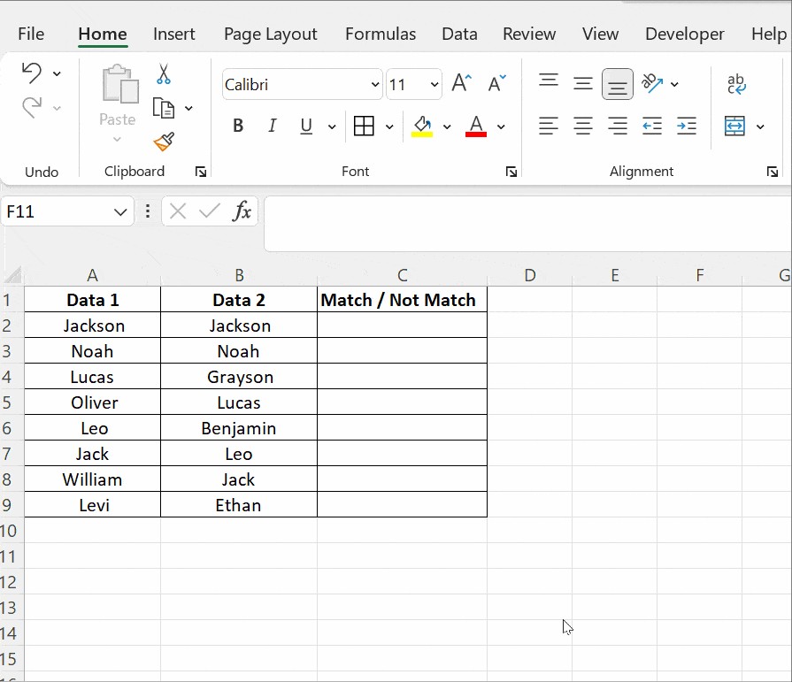
3.2. The IF Function: Adding Context with “Match” and “Mismatch”

The IF function allows you to add more context to your comparison by returning custom messages like “Match” or “Mismatch” instead of TRUE or FALSE.

Syntax: =IF(condition, value_if_true, value_if_false)

Steps:

1. In an empty column, enter the formula =IF(A2=B2, "Match", "Mismatch") and press Enter.
2. Drag the fill handle down to apply the formula to all rows.
3. The resulting column will display “Match” for matching rows and “Mismatch” for mismatched rows.

Example:

Column A	Column B	Column C (Formula: =IF(A2=B2, “Match”, “Mismatch”))
10	10	Match
25	30	Mismatch
15	15	Match
20	20	Match
35	40	Mismatch

3.3 Using the EXACT Function to Compare Two Columns

You can utilize the EXACT() function when comparing two columns in Excel and wish to find values that are case-sensitive.

The EXACT () function compares two text strings and returns TRUE if they are the same and FALSE otherwise. EXACT is case-sensitive but ignores formatting differences. The syntax is =EXACT( text1, text2). It takes two arguments, text1 and text2, and both are required arguments.

Let’s take a simple example. The columns data1 and data2 contain two text strings, Nova Scotia, in columns A and B.

The formula, =IF(A2=B2, “Match”, “Mismatch”), when applied to the cell C2, returns a match as it is case insensitive.

Use the formula =IF(EXACT(A2, B2), “Match”, “Mismatch”) for the IF condition to be case sensitive.

The EXACT() returns values as true or false. The execution of the formula would be: first, the inner function would be executed, and the result returned. In the above example, the EXACT() function returns a false value to the outer function IF.

The general working of the IF condition is that if it returns true, the first argument in the function is returned; else, the second argument is returned.

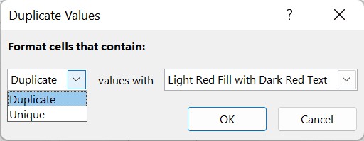
3.4. Conditional Formatting: Highlighting Matches and Differences

Conditional formatting allows you to visually highlight matches and differences between two columns based on specific criteria.

Steps:

1. Select the range of cells you want to format (e.g., both columns A and B).
2. Go to Home > Conditional Formatting > New Rule.
3. Choose “Use a formula to determine which cells to format.”
4. Enter the following formula to highlight matches: =A2=B2.
5. Click Format and choose a fill color or font style to indicate matches.
6. Click OK twice to apply the formatting.
7. Repeat steps 2-6 with the formula =A2<>B2 to highlight differences, choosing a different format to distinguish them from matches.

Example:

In this example, matching cells might be highlighted in green, while mismatched cells are highlighted in red.

3.5. COUNTIF: Identifying Duplicates and Unique Values

The COUNTIF function counts the number of cells within a range that meet a given criteria. This can be used to identify duplicates and unique values in two columns.

Syntax: =COUNTIF(range, criteria)

Steps:

1. To find duplicates, in an empty column, enter the formula =COUNTIF(B:B, A2) (assuming you want to check if values in column A exist in column B) and press Enter.
2. Drag the fill handle down to apply the formula to all rows in column A.
3. The resulting column will display the number of times each value in column A appears in column B. Values greater than 0 indicate duplicates.
4. To find unique values in column A that don’t exist in column B, use the formula =IF(COUNTIF(B:B, A2)=0, "Unique", ""). This will display “Unique” for values in column A that are not found in column B.

Example:

Column A	Column B	Column C (Formula: =COUNTIF(B:B, A2))	Column D (Formula: =IF(COUNTIF(B:B, A2)=0, “Unique”, “”))
10	20	0	Unique
25	10	1
15	30	0	Unique
20	25	1
35	40	0	Unique

3.6. VLOOKUP: Finding Matching Data Across Columns

VLOOKUP (Vertical Lookup) is a powerful function that searches for a value in the first column of a range and returns a corresponding value from another column in the same range. This can be useful for identifying matching data and retrieving related information.

Syntax: =VLOOKUP(lookup_value, table_array, col_index_num, [range_lookup])

• lookup_value: The value you want to search for.
• table_array: The range of cells where you want to search (the first column should contain the lookup_value).
• col_index_num: The column number in the table_array from which you want to retrieve the matching value.
• [range_lookup]: Optional. TRUE for approximate match, FALSE for exact match.

Steps:

1. Assuming you want to check if values in column A exist in column B and retrieve corresponding values from column B, enter the formula =VLOOKUP(A2, B:B, 1, FALSE) in an empty column and press Enter.
2. Drag the fill handle down to apply the formula to all rows in column A.
3. If a value in column A is found in column B, VLOOKUP will return the matching value from column B. If the value is not found, VLOOKUP will return #N/A.
4. You can use the ISNA function to handle #N/A errors and display a custom message like “Not Found”: =IF(ISNA(VLOOKUP(A2, B:B, 1, FALSE)), "Not Found", VLOOKUP(A2, B:B, 1, FALSE)).

Example:

Column A (Product ID)	Column B (Product ID)	Column C (Formula: =IF(ISNA(VLOOKUP(A2, B:B, 1, FALSE)), “Not Found”, VLOOKUP(A2, B:B, 1, FALSE)))
123	456	Not Found
456	789	456
789	123	789
012	901	Not Found
901	234	901

3.7. Combining Functions for Advanced Comparisons

You can combine different functions to perform more complex comparisons. For example, you can use the AND function to check if multiple conditions are met simultaneously.

Example:

To check if values in columns A and B are both greater than 10, use the formula =IF(AND(A2>10, B2>10), "Both Greater Than 10", "Not Both Greater Than 10").

4. Advanced Excel Comparison Techniques

Going beyond the basics, here are some advanced methods for comparing columns of numbers in Excel.

4.1. Array Formulas: Performing Calculations on Entire Ranges

Array formulas allow you to perform calculations on entire ranges of cells without having to enter individual formulas for each cell.

Example:

To compare two columns and return an array of TRUE/FALSE values indicating whether each row matches, you can use the array formula =(A1:A10=B1:B10). To enter an array formula, select the range where you want the results to appear, type the formula, and press Ctrl+Shift+Enter.

4.2. Using Power Query for Complex Data Transformations

Power Query is a powerful data transformation and analysis tool built into Excel. It allows you to import data from various sources, clean and transform it, and perform complex comparisons.

Steps:

1. Import your data into Power Query by going to Data > Get & Transform Data > From Table/Range.
2. Use Power Query’s transformation tools to clean and prepare your data for comparison.
3. To compare two columns, you can use the “Merge Queries” feature to join the two tables based on a common column.
4. After merging the tables, you can add a custom column that compares the values in the two columns and returns a TRUE/FALSE value.

4.3. VBA Macros: Automating Repetitive Comparison Tasks

VBA (Visual Basic for Applications) is a programming language that allows you to automate tasks in Excel. You can write VBA macros to perform complex comparisons and generate custom reports.

Example:

The following VBA macro compares two columns and highlights the differences in red:

Sub CompareColumns()
  Dim ws As Worksheet
  Dim lastRow As Long
  Dim i As Long

  Set ws = ThisWorkbook.Sheets("Sheet1") ' Replace "Sheet1" with your sheet name
  lastRow = ws.Cells(Rows.Count, "A").End(xlUp).Row ' Find the last row with data in column A

  For i = 2 To lastRow ' Start from row 2 (assuming row 1 is the header)
    If ws.Cells(i, "A").Value <> ws.Cells(i, "B").Value Then
      ws.Cells(i, "A").Interior.Color = RGB(255, 0, 0) ' Red
      ws.Cells(i, "B").Interior.Color = RGB(255, 0, 0) ' Red
    End If
  Next i
End Sub

To use this macro:

1. Press Alt+F11 to open the VBA editor.
2. Insert a new module by going to Insert > Module.
3. Paste the code into the module.
4. Modify the sheet name and column letters to match your data.
5. Run the macro by pressing F5 or clicking the “Run” button.

5. Practical Applications and Scenarios

Here are some real-world scenarios where comparing columns of numbers in Excel can be invaluable:

• Financial Analysis: Comparing actual vs. budget figures, tracking investment performance, and identifying fraudulent transactions.
• Sales and Marketing: Analyzing sales data across different regions, tracking customer acquisition costs, and measuring the effectiveness of marketing campaigns.
• Inventory Management: Comparing stock levels across different warehouses, identifying slow-moving items, and optimizing inventory levels.
• Scientific Research: Comparing experimental data across different groups, identifying statistically significant differences, and validating research findings.
• Quality Control: Comparing product measurements against specifications, identifying defects, and monitoring process variations.

6. Best Practices and Tips for Efficient Comparisons

To ensure accurate and efficient comparisons, follow these best practices:

• Clean and Prepare Your Data: Remove any inconsistencies, errors, or irrelevant data that could skew the results.
• Use Consistent Formatting: Ensure that the data in both columns is formatted consistently (e.g., number format, date format, text case).
• Handle Missing Values: Decide how to handle missing values (e.g., replace them with zeros, ignore them, or use a special indicator).
• Use Descriptive Column Headers: Clearly label your columns to make it easier to understand the data and the comparison results.
• Document Your Formulas: Add comments to your formulas to explain what they do and why you used them.
• Test Your Formulas: Verify that your formulas are working correctly by testing them with a small sample of data.
• Use Absolute References: Use absolute references ($) to prevent formulas from changing when you copy them to other cells.
• Consider Performance: When working with large datasets, use efficient formulas and techniques to minimize calculation time.

7. COMPARE.EDU.VN: Your Partner in Data Analysis

At COMPARE.EDU.VN, we understand the importance of data analysis and informed decision-making. That’s why we offer a range of resources and tools to help you master Excel and other data analysis techniques. Whether you’re a beginner or an experienced data analyst, our comprehensive guides, tutorials, and templates will empower you to unlock the full potential of your data.

We will assist you in discovering new ways to use data in Excel and offer simple techniques to analyze it.

8. Addressing Common Challenges and Pitfalls

Comparing columns of numbers in Excel can sometimes present challenges. Here are some common pitfalls to avoid:

• Inconsistent Data Types: Ensure that the data in both columns is of the same data type (e.g., numbers, text, dates).
• Hidden Characters: Watch out for hidden characters (e.g., spaces, non-printing characters) that can cause comparisons to fail.
• Rounding Errors: Be aware of rounding errors that can occur when working with decimal numbers.
• Case Sensitivity: Remember that some comparison functions (e.g., EXACT) are case-sensitive.
• Formula Errors: Double-check your formulas for syntax errors and logical mistakes.

If you encounter any of these challenges, take the time to troubleshoot your data and formulas to ensure accurate results.

9. The Future of Data Comparison in Excel

Excel is constantly evolving, with new features and capabilities being added regularly. Some of the trends that are shaping the future of data comparison in Excel include:

• AI-Powered Analysis: The integration of artificial intelligence (AI) and machine learning (ML) algorithms to automate data analysis and provide intelligent insights.
• Cloud-Based Collaboration: The ability to collaborate with others on Excel spreadsheets in real-time, making it easier to compare and analyze data together.
• Improved Data Visualization: The availability of more advanced data visualization tools to help you explore and communicate your findings more effectively.
• Enhanced Power Query Capabilities: The expansion of Power Query’s capabilities to support more complex data transformations and comparisons.
• Mobile Accessibility: The ability to access and analyze Excel data on mobile devices, allowing you to compare columns of numbers on the go.

By staying up-to-date with these trends, you can leverage the latest Excel features to improve your data comparison skills and gain a competitive edge.

10. FAQs: Quick Answers to Common Questions

1. How to compare two columns in Excel for differences?

Use the formula =IF(A2<>B2, "Different", "Same") to identify differences between two columns. You can also use conditional formatting to highlight differences visually.

2. How can I ignore case sensitivity when comparing two columns?

Use the UPPER or LOWER functions to convert both columns to the same case before comparing them. For example, =IF(UPPER(A2)=UPPER(B2), "Match", "Mismatch").

3. How do I compare two columns and return the values that are different?

Use the FILTER function to extract the values that are different. For example, =FILTER(A:A, A:A<>B:B).

4. Can I compare two columns in different Excel sheets?

Yes, you can use the same formulas and techniques to compare columns in different sheets. Just make sure to include the sheet name in your formula (e.g., =IF(Sheet1!A2=Sheet2!B2, "Match", "Mismatch")).

5. How to compare two columns in Excel and highlight the mismatched cells?

Select the range of cells, go to Home > Conditional Formatting > New Rule > Use a formula to determine which cells to format and enter the formula =A2<>B2. Then, choose a format to highlight the mismatched cells.

6. Is there a way to compare two columns for partial matches?

Use the SEARCH or FIND functions to check if one string is contained within another. For example, =IF(ISNUMBER(SEARCH(A2, B2)), "Partial Match", "No Match").

7. How can I compare two columns and count the number of matches?

Use the SUMPRODUCT function along with a comparison formula. For example, =SUMPRODUCT(--(A1:A10=B1:B10)) will count the number of matching rows in the range A1:A10 and B1:B10.

8. How do I compare two columns and find the largest difference?

Use the MAX and ABS functions to find the largest absolute difference. For example, =MAX(ABS(A1:A10-B1:B10)).

9. How to compare two columns and return corresponding values from a third column based on matches?

Use the INDEX and MATCH functions together. For example, if you want to return values from column C when columns A and B match, use the formula =INDEX(C:C, MATCH(A2, B:B, 0)).

10. What is the best way to compare two very large columns in Excel?

Consider using Power Query or VBA macros to optimize performance and handle large datasets more efficiently.

11. Next Steps: Putting Your Knowledge into Action

Now that you’ve learned the different techniques for comparing two columns of numbers in Excel, it’s time to put your knowledge into action. Start by practicing with sample datasets and gradually move on to more complex real-world scenarios.

Remember, COMPARE.EDU.VN is here to support you every step of the way. Visit our website at COMPARE.EDU.VN for more resources, tutorials, and templates to help you master Excel and data analysis.

Address: 333 Comparison Plaza, Choice City, CA 90210, United States

Whatsapp: +1 (626) 555-9090

Conclusion: Empowering You to Make Data-Driven Decisions

Comparing two columns of numbers in Excel is a fundamental skill for data analysis and informed decision-making. By mastering the techniques outlined in this guide, you’ll be able to:

• Validate data and identify discrepancies
• Analyze trends and patterns
• Evaluate performance and track progress
• Make data-driven decisions with confidence

Don’t let the complexities of data analysis hold you back. With the right knowledge and tools, you can unlock the hidden insights within your spreadsheets and gain a competitive edge.

Visit compare.edu.vn today and discover how we can help you take your data analysis skills to the next level. Our comprehensive resources and expert guidance will empower you to make smarter, faster, and more informed decisions. Let us help you in your data analysis and data needs.