Finding duplicate entries across two columns in Google Sheets can be a tedious task. Fortunately, Google Sheets provides a powerful feature called Conditional Formatting, allowing you to quickly identify and highlight these duplicates. This article provides a step-by-step guide on how to compare two columns in Google Sheets for duplicates and customize the highlighting for easy identification.
Identifying Duplicates Across Two Columns
1. Define the Range
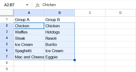
Start by selecting the two columns you want to compare. If the range is small, you can simply click and drag your cursor over the cells. For larger ranges, noting the cell coordinates (e.g., A1:B10) is more efficient. This range will be used in the subsequent steps.
2. Access Conditional Formatting
In the Google Sheets menu bar, navigate to Format > Conditional formatting. This will open the Conditional format rules sidebar on the right side of your screen.
3. Utilize a Custom Formula
Within the Conditional format rules sidebar, under “Format rules”, choose “Custom formula is” from the dropdown menu. This allows you to apply formatting based on a specific formula.
4. Implement the COUNTIF Formula
In the formula textbox, enter the following formula: =COUNTIF(range, first_cell)>1.
- range: Replace this with the absolute reference of the range you defined in Step 1 (e.g., $A$1:$B$10). Absolute references ensure the formula applies to the correct cells even when copied.
- first_cell: Replace this with the first cell in your range (e.g., A1). This cell will be compared to all other cells in the range.
For example, if your range is A1:B10, the formula would be: =COUNTIF($A$1:$B$10,A1)>1. This formula counts how many times the value in A1 appears in the range A1:B10. If the count is greater than 1, it indicates a duplicate.
5. Apply the Formatting
Once you’ve entered the formula, click “Done”. Google Sheets will now highlight any duplicate entries found across the two columns.
This method efficiently identifies duplicate entries, enabling you to clean and manage your data effectively. You can customize the highlight color by clicking the fill color icon and choosing your preferred color. This process can be easily extended to compare more than two columns by adjusting the range in the COUNTIF formula.