How to Compare Two Columns in Excel VLOOKUP

Comparing data across two Excel columns is a common task for many. Whether you need to identify matching entries, find discrepancies, or extract corresponding values, Excel’s VLOOKUP function provides a powerful solution. This guide will delve into various techniques using VLOOKUP to compare two columns in Excel, empowering you to efficiently analyze and manipulate your data.

Using VLOOKUP to Find Common Values

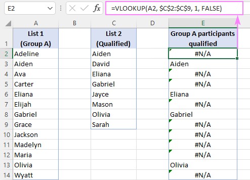
VLOOKUP allows you to search for a specific value in the first column of a range (your lookup table) and return a corresponding value from another column in the same row. To compare two columns (let’s say column A and column C) for common values:

Enter the VLOOKUP formula: In a new column (e.g., column E), enter the following formula in the first cell (E2): =VLOOKUP(A2,$C$2:$C$9,1,FALSE). This formula searches for the value in A2 within the range C2:C9. The 1 signifies that the return value should be from the first column of the lookup range (which is column C in this case), and FALSE ensures an exact match. Remember to use absolute references ($) for the lookup range so it remains fixed when copying the formula.
Copy the formula down: Drag the fill handle (the small square at the bottom right of the cell) down to apply the formula to all rows in column A.
Interpret the results: If a value from column A is found in column C, the corresponding value from column C will be displayed in column E. If a value is not found, the formula will return #N/A.

Handling #N/A Errors

To make the results cleaner and more user-friendly, you can replace #N/A errors with blank cells or custom text:

Blank cells: Use the IFNA function: =IFNA(VLOOKUP(A2,$C$2:$C$9,1,FALSE),"").
Custom text: =IFNA(VLOOKUP(A2,$C$2:$C$9,1,FALSE),"Not Found").

Comparing Columns in Different Sheets

To compare columns across different sheets, simply include the sheet name in the table array argument:

=IFNA(VLOOKUP(A2,Sheet2!$A$2:$A$9,1,FALSE),"")

Isolating Matches and Differences

Finding only matches: Filter the results column to exclude #N/A values or blanks. Alternatively, use the FILTER function in Excel 365/2021: =FILTER(A2:A14,IFNA(VLOOKUP(A2:A14,C2:C9,1,FALSE),"")<>"")

Finding only differences: Use the ISNA function with IF: =IF(ISNA(VLOOKUP(A2,$C$2:$C$9,1,FALSE)),A2,""). This formula returns values from column A that are not found in column C. Again, filtering or the FILTER function can be used to isolate these differences.

Returning Values from a Third Column

VLOOKUP’s true power lies in its ability to retrieve related data. To compare two columns (A and D) and return a value from a third column (E) based on matches: =IFNA(VLOOKUP(A2,$D$2:$E$9,2,FALSE),""). The 2 in the formula indicates that the return value should be from the second column of the lookup range (column E).

Conclusion

VLOOKUP is a versatile tool for comparing data in Excel. By understanding its core functionality and combining it with other functions like IFNA, ISNA, and FILTER, you can efficiently perform various comparison tasks, from finding matches and differences to extracting related information. Mastering these techniques will significantly enhance your data analysis capabilities in Excel.