Comparing data in Excel is a fundamental skill, especially when dealing with large datasets. This guide focuses on how to compare two columns in Excel for true false results, providing clear explanations and practical examples to help you master various techniques. We’ll cover using formulas, conditional formatting, and lookup functions to efficiently compare your data and get the insights you need.
Comparing Columns in Excel: A Comprehensive Guide
Excel offers several methods for comparing columns and identifying matches or discrepancies. Choosing the right technique depends on your specific needs and the complexity of your data. Here, we will explore the most effective methods for generating true/false results when comparing two columns.
Using the Equals Operator for Direct Comparison
The simplest way to compare two columns row by row is using the equals operator (=). In a new column, enter a formula like =A2=B2. This formula compares the values in cells A2 and B2 and returns TRUE if they are identical, and FALSE if they are different. Drag this formula down to apply it to all rows in your data.
Leveraging the IF Function for Customized Results
The IF function provides more flexibility, allowing you to specify custom outputs for true and false results. For instance, the formula =IF(A2=B2,"Match","No Match") returns “Match” for identical values and “No Match” for different values. You can tailor the output to your specific requirements. For a simple true/false output, use =IF(A2=B2,TRUE,FALSE).
Case-Sensitive Comparisons with the EXACT Function
For text comparisons where case sensitivity matters, use the EXACT function. The formula =EXACT(A2,B2) returns TRUE only if the text in A2 and B2 is identical, including case. Otherwise, it returns FALSE. Combine this with the IF function for custom outputs: =IF(EXACT(A2,B2),"Match","No Match").
Visualizing Comparisons with Conditional Formatting
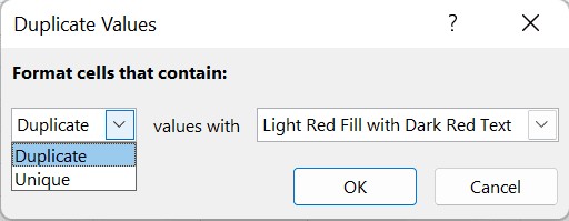
Conditional formatting highlights cells based on specific criteria, providing a visual representation of your comparison results. Select the two columns you want to compare, go to Home > Conditional Formatting > Highlight Cells Rules > Duplicate Values. Choose a formatting style to highlight matching or unique values. While this doesn’t directly provide true/false values, it offers a quick visual overview of similarities and differences.
Advanced Comparisons with VLOOKUP
The VLOOKUP function searches for a specific value in one column and returns a corresponding value from another column. This is useful for comparing data across different tables or sheets. While VLOOKUP doesn’t directly return true/false, it can indicate whether a value exists in another column. If a match is found, VLOOKUP returns the corresponding value; otherwise, it returns an error (#N/A). You can use =IFERROR(VLOOKUP(A2,B:B,1,FALSE),"No Match") to return “No Match” when a value isn’t found.
Conclusion
This guide has provided a range of techniques for comparing two columns in Excel and obtaining true/false results. From simple formulas to more advanced functions and visual comparisons, you now have the tools to analyze your data effectively and extract valuable insights. Choose the method that best suits your needs and data structure, and remember to practice to solidify your understanding.

