Master Excel: How to Compare Two Columns for Matches

In the world of data analysis, Microsoft Excel stands as a powerful tool for organizing, manipulating, and interpreting information. Often, working with spreadsheets involves comparing datasets to identify similarities, differences, or overlaps. A common task is to compare two columns in Excel for matches. Whether you’re managing inventory, reconciling financial records, or cleaning customer lists, efficiently comparing columns is a crucial skill.

Manually sifting through rows of data to find matches is not only tedious but also prone to errors, especially with large datasets. Fortunately, Excel provides a range of built-in features and formulas to automate this process, saving you time and ensuring accuracy.

This comprehensive guide will walk you through various methods to effectively compare two columns in Excel to find matches. We’ll explore techniques ranging from simple operators to more advanced functions and conditional formatting, equipping you with the knowledge to choose the best approach for your specific needs. Whether you’re a beginner or an experienced Excel user, you’ll discover valuable strategies to streamline your data analysis workflow and unlock deeper insights from your spreadsheets.

Why Comparing Columns in Excel is Essential

Excel’s strength lies in its ability to handle and analyze data effectively. Comparing columns within Excel spreadsheets is not just a convenience; it’s a fundamental operation for numerous data-driven tasks. Here’s why it’s so useful:

• Data Validation and Cleaning: Ensure data consistency across different sources or within the same dataset. Identify discrepancies, duplicates, or missing entries that need correction.
• Identifying Common Data Points: Discover shared items between lists, such as matching customer IDs across different databases, or common products in inventory lists.
• Reconciliation and Auditing: Verify the accuracy of records by comparing transaction lists, financial statements, or inventory counts against expected values.
• Data Integration: Merge or combine datasets by identifying common keys or identifiers in different columns, enabling seamless data integration.
• Tracking Changes Over Time: Compare datasets from different periods to monitor changes, trends, and growth patterns.

Without the ability to efficiently compare columns, these tasks would become incredibly time-consuming and error-prone. Excel’s column comparison features empower users to work with data more effectively, make informed decisions, and extract meaningful insights.

Methods to Compare Two Columns in Excel for Matches

Excel offers several methods to compare two columns and highlight or extract matching data. The best method depends on your specific requirements, such as whether you need to simply highlight matches, return a “Match” or “No Match” result, or extract the matching values themselves. Here are some of the most effective techniques:

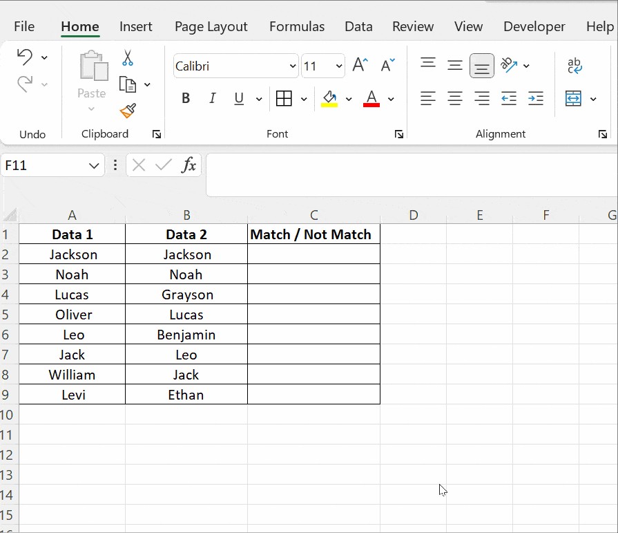
1. Using the Equals Operator (=) for Row-by-Row Comparison

The simplest method to compare two columns is to use the equals operator (=) for a row-by-row comparison. This method is ideal for quickly identifying matching entries in corresponding rows of two columns.

Steps:

1. In an empty column next to your data (e.g., Column C if your data is in Columns A and B), in the first cell of that column (e.g., C2), enter the formula =A2=B2.
2. Press Enter. The cell will display TRUE if the values in cells A2 and B2 are identical, and FALSE otherwise.
3. Drag the fill handle (the small square at the bottom-right of the cell C2) down to apply the formula to the rest of the rows in your data.

Explanation:

• A2=B2 directly compares the value in cell A2 with the value in cell B2.
• Excel returns a logical value: TRUE for a match, FALSE for a mismatch.

Pros:

• Very simple and quick to implement.
• Provides immediate TRUE/FALSE results for each row.

Cons:

• Only shows TRUE/FALSE. Doesn’t provide more descriptive outputs like “Match” or “Mismatch”.
• Case-insensitive comparison. “Apple” and “apple” are considered a match.

2. Using the IF Function for “Match” or “No Match” Results

To get more user-friendly results than TRUE/FALSE, you can combine the equals operator with the IF function. This allows you to display custom text like “Match” or “No Match”.

Steps:

1. In an empty column (e.g., Column C), in the first cell (e.g., C2), enter the formula =IF(A2=B2,"Match","No Match").
2. Press Enter and drag the fill handle down to apply the formula to the rest of the rows.

Explanation:

• IF(A2=B2,"Match","No Match") checks if A2=B2 is TRUE.
  • If TRUE (values match), it returns “Match”.
  • If FALSE (values don’t match), it returns “No Match”.

Formula Variations:

• To leave mismatching rows blank: =IF(A2=B2,"Match","")
• To find mismatches (show “Match” for differences): =IF(A2<>B2,"Mismatch","Match") (using the “not equal to” operator <>)

Pros:

• Provides more descriptive results than TRUE/FALSE.
• Customizable output text.
• Still relatively simple to use.

Cons:

• Case-insensitive comparison.
• Row-by-row comparison only.

3. Using the EXACT Function for Case-Sensitive Comparisons

If you need to perform a case-sensitive comparison, the EXACT function is the perfect tool. It compares two text strings and returns TRUE only if they are exactly the same, including case.

Steps:

1. In an empty column (e.g., Column C), in the first cell (e.g., C2), enter the formula =IF(EXACT(A2,B2),"Match","No Match").
2. Press Enter and drag the fill handle down.

Explanation:

• EXACT(A2,B2) compares the text in cell A2 and cell B2 case-sensitively.
• The IF function then uses the TRUE/FALSE result from EXACT to display “Match” or “No Match”.

Pros:

• Performs case-sensitive comparisons.
• Useful when case sensitivity is important for data accuracy.

Cons:

• Slightly more complex formula than the equals operator alone.
• Still row-by-row comparison.

4. Conditional Formatting to Highlight Matches or Differences

Conditional formatting provides a visual way to highlight matching or unique values directly within your columns, without needing a separate results column.

Steps:

1. Select the columns you want to compare (e.g., Columns A and B).
2. Go to the Home tab on the Excel ribbon.
3. Click on Conditional Formatting in the Styles group.
4. Choose Highlight Cells Rules and then Duplicate Values…

5. In the Duplicate Values dialog box:
   • In the dropdown menu on the left, ensure Duplicate is selected if you want to highlight matches. Choose Unique if you want to highlight differences.
   • Choose a formatting style from the “with” dropdown (e.g., “Light Red Fill with Dark Red Text”) or select “Custom Format…” for more options.
6. Click OK.

Explanation:

• Duplicate Values rule highlights cells that appear more than once within the selected range. When applied to both columns simultaneously, it highlights values that are present in both columns.
• Unique Values rule highlights cells that appear only once within the selected range, effectively highlighting values that are different between the two columns within the combined selection.

Pros:

• Visually highlights matches or differences directly in the columns.
• No need for formulas or extra columns.
• Easy to apply and customize formatting.

Cons:

• Highlights all duplicates or uniques within the selected range, not just between the two columns specifically if you select both columns together. For more precise column-to-column matching highlighting, consider using formulas with conditional formatting.
• Primarily visual; doesn’t return text results like “Match” or “No Match”.

To Highlight Matches in Column A Based on Column B:

To highlight values in Column A that are also present in Column B, you can use a formula-based conditional formatting rule:

1. Select Column A.
2. Go to Home > Conditional Formatting > New Rule…
3. Choose “Use a formula to determine which cells to format”.
4. Enter the formula: =COUNTIF($B:$B,A1)>0
5. Click Format… and choose your desired highlighting style.
6. Click OK twice.

Explanation of the formula:

• COUNTIF($B:$B,A1): Counts how many times the value in cell A1 appears in the entire Column B ($B:$B).
• >0: Checks if the count is greater than zero, meaning the value from A1 is found at least once in Column B.
• If the condition is TRUE, the conditional formatting is applied to cell A1 (and subsequently to all cells in Column A based on their respective values).

5. Using VLOOKUP for Finding Matches and Extracting Related Data

The VLOOKUP function is a powerful tool for comparing columns and, more importantly, for finding matches in one column (the lookup column) and retrieving corresponding data from another column (or table). While primarily designed for lookups, it can be adapted to identify matches between two columns.

Steps (to check if values in Column A exist in Column B):

1. In an empty column (e.g., Column C), in the first cell (e.g., C2), enter the formula =IF(ISNA(VLOOKUP(A2,$B:$B,1,FALSE)),"No Match","Match").
2. Press Enter and drag the fill handle down.

Explanation:

• VLOOKUP(A2,$B:$B,1,FALSE):
  • A2: The lookup value (the value from Column A you are searching for in Column B).
  • $B:$B: The lookup table or range (Column B in this case). $B:$B uses absolute referencing to keep the column fixed when dragging the formula.
  • 1: The column index number (we’re just checking for existence, so we can use 1, as we are essentially looking up in a single column range).
  • FALSE: Specifies an exact match (essential for accurate comparison).
• ISNA(VLOOKUP(...)): Checks if VLOOKUP returns #N/A. VLOOKUP returns #N/A if it cannot find the lookup value.
• IF(ISNA(...),"No Match","Match"): If ISNA is TRUE (meaning VLOOKUP returned #N/A, no match found), it displays “No Match”. Otherwise (a match was found), it displays “Match”.

Pros:

• Can identify matches and simultaneously retrieve related data if your lookup range has multiple columns.
• Versatile and widely used function in Excel.
• Can be adapted for more complex lookup scenarios.

Cons:

• More complex formula compared to simpler methods.
• Can be slightly slower for very large datasets compared to basic operators.

Frequently Asked Questions

1. How can I compare two columns in Excel and highlight the rows that are different?

You can use conditional formatting with a formula to highlight entire rows where columns are different. Select your data range, then create a new conditional formatting rule using a formula like =A1<>B1 (adjust cell references as needed). Choose a formatting style to apply to the rows where this condition is true.

2. Can I compare two columns in different Excel sheets?

Yes, you can compare columns across different sheets. In your formulas, simply reference the columns using the sheet name followed by an exclamation mark and the column range. For example, to compare Column A in Sheet1 with Column A in Sheet2, you might use a formula like =IF(Sheet1!A2=Sheet2!A2,"Match","No Match") in a third sheet or in one of the existing sheets.

3. What if my columns have different lengths?

When comparing columns of different lengths, formulas like the equals operator and IF function will only compare up to the length of the shorter column when dragged down. For more advanced scenarios, you might need to adjust formulas or use VBA if you need to handle mismatches in length systematically. For basic match finding, the methods described will still work for the overlapping portion of the columns.

4. How do I compare two columns and find only the unique values in each column (values that are in one column but not the other)?

Conditional formatting with “Unique Values” can highlight unique entries within the selected range. To find unique values between two columns, you might need to use more complex formulas involving COUNTIF or MATCH to check for the absence of values in the other column, or consider using Power Query for more advanced data shaping and comparison tasks.

Conclusion

Comparing two columns in Excel for matches is a fundamental data analysis task, and Excel offers a variety of methods to accomplish this efficiently. From simple equals operators and IF conditions to the more powerful EXACT, conditional formatting, and VLOOKUP functions, you have a toolkit to handle various comparison needs.

By mastering these techniques, you can significantly improve your data analysis workflow, ensure data accuracy, and extract valuable insights from your spreadsheets. Choose the method that best suits your specific requirements and data complexity, and unlock the full potential of Excel for data comparison.