**How to Compare Two Columns in Excel Using VLOOKUP: A Comprehensive Guide**

Comparing two columns in Excel is a common task for data analysis, list management, and ensuring data integrity. This comprehensive guide, brought to you by COMPARE.EDU.VN, demonstrates How To Compare Two Columns In Excel By Using Vlookup along with alternative methods for identifying matching values, missing data, and associated data. Whether you’re a student, professional, or data enthusiast, this article equips you with the knowledge to efficiently analyze and compare data sets within Excel, enhancing your productivity and decision-making capabilities. Learn how to use VLOOKUP for data comparison, master IFNA and FILTER functions, and discover advanced techniques for effective data analysis.

1. Understanding the Basics of VLOOKUP for Column Comparison

VLOOKUP (Vertical Lookup) is an Excel function that searches for a value in the first column of a range and returns a value in the same row from another column in the range. When comparing two columns, VLOOKUP can identify whether values from one column exist in another. This is a fundamental technique for data validation and reconciliation.

1.1. Syntax and Arguments of VLOOKUP

The VLOOKUP function has the following syntax:

VLOOKUP(lookup_value, table_array, col_index_num, [range_lookup])

lookup_value: The value to search for in the first column of the table_array.
table_array: The range of cells in which to search. The first column of this range is where the lookup_value is searched.
col_index_num: The column number in the table_array from which to return a matching value.
range_lookup: An optional argument that specifies whether to find an exact match (FALSE) or an approximate match (TRUE). For comparing columns, it is usually set to FALSE for exact matches.

1.2. Simple Example: Identifying Common Values

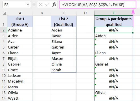
Consider two lists: List 1 in column A and List 2 in column C. To find which values from List 1 are present in List 2, use the following formula in column E:

=VLOOKUP(A2, $C$2:$C$9, 1, FALSE)

This formula searches for the value in A2 within the range C2:C9. If a match is found, it returns the value from the first column of the range (which is the matching value itself). If no match is found, it returns a #N/A error.

1.3. Handling #N/A Errors with IFNA and IFERROR

The #N/A error can be unsightly and confusing. To replace these errors with more user-friendly outputs, use the IFNA or IFERROR functions.

IFNA: Specifically designed to handle #N/A errors.

=IFNA(VLOOKUP(A2, $C$2:$C$9, 1, FALSE), "")

This formula returns an empty string (“”) if VLOOKUP results in a #N/A error, effectively displaying a blank cell. You can replace “” with any desired text, such as “Not Found”.
IFERROR: More general, catching all types of errors, not just #N/A.

=IFERROR(VLOOKUP(A2, $C$2:$C$9, 1, FALSE), "")

While IFERROR works, IFNA is preferable in this context because it specifically targets #N/A errors, ensuring other potential errors are not masked.

2. Comparing Columns Across Different Excel Sheets

Often, the columns you need to compare reside in different sheets within the same Excel workbook. VLOOKUP can easily handle this scenario using external references.

2.1. Creating External References

To reference a range in another sheet, simply include the sheet name followed by an exclamation mark (!) before the cell range. For example, if List 1 is in column A of “Sheet1” and List 2 is in column A of “Sheet2”, the formula would be:

=IFNA(VLOOKUP(A2, Sheet2!$A$2:$A$9, 1, FALSE), "")

2.2. Step-by-Step Guide to Comparing Columns in Different Sheets

Open the Excel workbook containing the sheets you want to compare.
Select the sheet where you want to display the comparison results (e.g., Sheet1).
Enter the VLOOKUP formula in the desired cell (e.g., B2), referencing the other sheet:
=IFNA(VLOOKUP(A2, Sheet2!$A$2:$A$9, 1, FALSE), "")
Drag the formula down to apply it to the rest of the column.
Review the results. Matching values from Sheet1 that are found in Sheet2 will be displayed; otherwise, the specified error replacement (e.g., “”) will appear.

3. Advanced Techniques: Returning Common and Missing Values

Beyond basic comparison, VLOOKUP can be used to extract specific data: common values (matches) and missing values (differences).

3.1. Returning Common Values (Matches)

The basic VLOOKUP formula returns a list with matching values and #N/A errors (or their replacements). To isolate only the common values without gaps, use Excel’s filtering capabilities or dynamic array functions.

3.1.1. Using Auto-Filter

Apply the VLOOKUP formula: =IFNA(VLOOKUP(A2, $C$2:$C$9, 1, FALSE), "") in column E.
Select the header of column E (e.g., E1).
Go to the “Data” tab in the Excel ribbon and click “Filter”.
Click the filter dropdown in the header of column E.
Uncheck the “Blanks” option. This will display only the rows with matching values.

3.1.2. Using the FILTER Function (Excel 365 and 2021)

For dynamic arrays, the FILTER function provides a more efficient solution:

=FILTER(A2:A14, IFNA(VLOOKUP(A2:A14, C2:C9, 1, FALSE), "")<>"")

This formula filters the range A2:A14, including only values for which the VLOOKUP function finds a match (i.e., not replaced by “”).

Alternatively, using ISNA:

=FILTER(A2:A14, ISNA(VLOOKUP(A2:A14, C2:C9, 1, FALSE))=FALSE)

This formula filters the range A2:A14, including only values for which VLOOKUP does not return a #N/A error (i.e., a match is found).

3.1.3. Using the XLOOKUP Function (Excel 365 and 2021)

XLOOKUP, the modern successor to VLOOKUP, simplifies the formula further:

=FILTER(A2:A14, XLOOKUP(A2:A14, C2:C9, C2:C9,"")<>"")

XLOOKUP’s ability to handle #N/A errors internally eliminates the need for IFNA or ISNA.

3.2. Returning Missing Values (Differences)

To identify values that are present in List 1 but not in List 2, use a combination of IF and ISNA with VLOOKUP.

3.2.1. Using IF and ISNA

=IF(ISNA(VLOOKUP(A2, $C$2:$C$9, 1, FALSE)), A2, "")

This formula checks if VLOOKUP returns a #N/A error (using ISNA). If it does, the formula returns the value from List 1 (A2); otherwise, it returns an empty string.

To filter out the blanks and display only the missing values, use Auto-Filter as described earlier.

3.2.2. Using the FILTER Function (Excel 365 and 2021)

For dynamic arrays, the FILTER function offers a streamlined approach:

=FILTER(A2:A14, ISNA(VLOOKUP(A2:A14, C2:C9, 1, FALSE)))

This formula filters the range A2:A14, including only values for which VLOOKUP returns a #N/A error (i.e., missing values).

Alternatively, using XLOOKUP:

=FILTER(A2:A14, XLOOKUP(A2:A14, C2:C9, C2:C9,"")="")

This formula filters the range A2:A14, including only values for which XLOOKUP returns an empty string (i.e., missing values).

4. Labeling Matches and Differences for Clarity

For enhanced readability, you can add text labels to indicate whether a value is a match or a difference.

4.1. Using IF, ISNA/ISERROR, and VLOOKUP

=IF(ISNA(VLOOKUP(A2, $D$2:$D$9, 1, FALSE)), "Not in List 2", "In List 2")

This formula checks if VLOOKUP returns a #N/A error. If it does, the formula returns “Not in List 2”; otherwise, it returns “In List 2”.

4.2. Using MATCH Function

Alternatively, the MATCH function can be used:

=IF(ISNA(MATCH(A2, $D$2:$D$9, 0)), "Not in List 2", "In List 2")

This formula checks if the MATCH function returns a #N/A error. If it does, the formula returns “Not in List 2”; otherwise, it returns “In List 2”.

5. Returning Values from a Third Column Based on Comparison

VLOOKUP’s primary strength lies in its ability to return a value from a third column based on a match in the lookup.

5.1. Basic VLOOKUP to Return Associated Data

Consider two tables: one with names in column A and another with names in column D and corresponding times in column E. To return the time from column E for matching names in column A, use:

=VLOOKUP(A2, $D$2:$E$10, 2, FALSE)

This formula searches for the name in A2 within the range D2:E10 and returns the value from the second column of the range (column E), which is the corresponding time.

5.2. Handling Errors and Filtering Results

To handle #N/A errors, use IFNA:

=IFNA(VLOOKUP(A2, $D$2:$E$10, 2, FALSE), "Not Available")

This formula returns “Not Available” if no match is found.

For more flexibility, the INDEX MATCH combination is powerful:

=IFNA(INDEX($E$2:$E$10, MATCH(A2, $D$2:$D$10, 0)), "Not Available")

This formula first uses MATCH to find the row number of the matching name and then uses INDEX to return the corresponding time.

XLOOKUP provides a modern, more concise alternative:

=XLOOKUP(A2, $D$2:$D$10, $E$2:$E$10, "Not Available")

Finally, to filter out entries without times, use the FILTER function:

=FILTER(A2:B14, B2:B14<>"")

This formula filters the range A2:B14, including only rows where the time is not blank.

6. Alternatives to VLOOKUP for Column Comparison

While VLOOKUP is a powerful tool, Excel offers several alternatives for comparing columns, each with its strengths and weaknesses.

6.1. MATCH Function

The MATCH function returns the position of a value in a range. It can be used to check if a value exists in another column:

=ISNUMBER(MATCH(A2, $C$2:$C$9, 0))

This formula returns TRUE if the value in A2 is found in the range C2:C9 and FALSE otherwise.

6.2. COUNTIF Function

The COUNTIF function counts the number of cells within a range that meet a given criterion. It can be used to check if a value exists in another column:

=COUNTIF($C$2:$C$9, A2)>0

This formula returns TRUE if the value in A2 exists at least once in the range C2:C9 and FALSE otherwise.

6.3. Conditional Formatting

Conditional formatting can highlight matching or different values directly in the columns:

Select the range of cells you want to compare (e.g., A2:A14).
Go to the “Home” tab in the Excel ribbon and click “Conditional Formatting”.
Choose “New Rule…”.
Select “Use a formula to determine which cells to format”.
Enter a formula to highlight matches or differences. For example, to highlight matches with List 2:

=COUNTIF($C$2:$C$9, A2)>0
Click “Format…” and choose the desired formatting (e.g., fill color).
Click “OK” to apply the conditional formatting.

6.4. Power Query

Power Query is a powerful data transformation and analysis tool built into Excel. It can be used to compare columns and merge data from different sources.

Select the data in each column.
Go to the “Data” tab and click “From Table/Range”.
In the Power Query Editor, perform merges or comparisons as needed.
Load the results back into Excel.

7. Optimizing VLOOKUP Performance

When working with large datasets, VLOOKUP performance can be a concern. Here are some tips to optimize VLOOKUP:

Sort the lookup column: Sorting the first column of the table_array can significantly speed up VLOOKUP, especially when using approximate matches (though this is less relevant for exact matches, which are typically used for column comparison).
Use absolute references: Ensure that the table_array is locked with absolute references ($) to prevent it from shifting when the formula is copied.
Minimize the table_array size: Keep the table_array as small as possible to reduce the amount of data VLOOKUP needs to search through.
Consider alternatives: For very large datasets, consider using INDEX MATCH or Power Query, which may offer better performance.

8. Real-World Applications of Column Comparison

Comparing columns in Excel has numerous practical applications across various domains:

Data Validation: Ensuring that data entered into one column matches the expected values in another column.
Reconciliation: Comparing financial data between two systems to identify discrepancies.
Inventory Management: Comparing stock levels between a database and a physical count.
Customer Relationship Management (CRM): Identifying duplicate customer records.
HR Management: Comparing employee data across different departments or systems.
Academic Research: Comparing data sets for statistical analysis.

9. Best Practices for Data Comparison in Excel

To ensure accurate and efficient data comparison, follow these best practices:

Clean your data: Remove duplicates, correct errors, and standardize formats before comparing columns.
Use consistent formulas: Ensure that the VLOOKUP or other comparison formulas are applied consistently across all rows.
Test your formulas: Verify that your formulas are working correctly by testing them with known data.
Document your process: Keep a record of the steps you took to compare columns, including the formulas used and any data transformations performed.
Use clear labels: Label your columns and results clearly to avoid confusion.
Consider data volume: Choose the appropriate method for the size of your data. For large datasets, consider Power Query or other advanced techniques.

10. Advanced Formulas and Functions for Data Analysis

To enhance your data analysis skills, explore these advanced Excel formulas and functions:

INDEX and MATCH: A flexible alternative to VLOOKUP that can handle more complex lookups.
OFFSET: Returns a reference to a range that is a specified number of rows and columns from a starting cell.
INDIRECT: Converts a text string into a valid cell reference.
SUMIFS, AVERAGEIFS, COUNTIFS: Perform calculations based on multiple criteria.
GETPIVOTDATA: Extracts data from a PivotTable.
AGGREGATE: Returns an aggregate calculation while ignoring errors and hidden rows.

11. Addressing Common Issues and Troubleshooting

When using VLOOKUP and other comparison techniques, you may encounter some common issues:

#N/A errors: Ensure that the lookup_value exists in the first column of the table_array.
Incorrect results: Double-check that the col_index_num is correct and that the table_array is properly defined.
Performance issues: Optimize your formulas and consider using alternative methods for large datasets.
Data type mismatches: Ensure that the data types of the lookup_value and the values in the first column of the table_array are compatible.
Case sensitivity: VLOOKUP is not case-sensitive. To perform a case-sensitive lookup, use the FIND function in combination with other functions.

12. Leveraging COMPARE.EDU.VN for Informed Decisions

At COMPARE.EDU.VN, we understand the challenges of making informed decisions in a world of abundant choices. Our mission is to provide you with comprehensive, objective comparisons across various products, services, and ideas. Whether you’re a student, professional, or consumer, our platform equips you with the insights you need to make confident decisions.

12.1. How COMPARE.EDU.VN Simplifies Decision-Making

Objective Comparisons: We provide unbiased comparisons based on thorough research and analysis.
Detailed Information: Our comparisons include key features, specifications, pros and cons, and user reviews.
User-Friendly Interface: Our website is designed to be intuitive and easy to navigate, making it simple to find the comparisons you need.
Wide Range of Categories: We cover a broad range of categories, including technology, education, finance, and more.

12.2. Benefits of Using COMPARE.EDU.VN

Save Time and Effort: Avoid spending hours researching and comparing options on your own.
Make Informed Decisions: Get the information you need to choose the best option for your needs.
Reduce Risk: Minimize the risk of making a poor decision by relying on our objective comparisons.
Increase Confidence: Feel confident that you’ve made the right choice.

13. Case Studies: Real-World Examples of VLOOKUP in Action

To illustrate the power of VLOOKUP, let’s examine some real-world case studies:

13.1. Case Study 1: Sales Data Analysis

A sales manager wants to compare the sales data from two different systems to identify any discrepancies. By using VLOOKUP to compare customer IDs and sales amounts, the manager can quickly identify any missing or mismatched data.

13.2. Case Study 2: Inventory Management

A warehouse manager needs to reconcile the inventory data in a database with a physical count. By using VLOOKUP to compare product codes and quantities, the manager can identify any stock level discrepancies.

13.3. Case Study 3: Customer Relationship Management (CRM)

A marketing team wants to identify duplicate customer records in a CRM system. By using VLOOKUP to compare customer names and email addresses, the team can merge duplicate records and improve data quality.

14. Additional Resources and Learning Materials

To further enhance your Excel skills, explore these additional resources:

Microsoft Excel Help: The official Excel documentation from Microsoft.
Excel Forums: Online communities where you can ask questions and get help from other Excel users.
Excel Blogs: Websites and blogs that offer tips, tricks, and tutorials on Excel.
Online Courses: Online courses on platforms like Coursera, Udemy, and LinkedIn Learning.
Books: Books on Excel from reputable publishers.

15. Frequently Asked Questions (FAQ)

1. What is VLOOKUP used for?

VLOOKUP is used to search for a value in the first column of a range and return a value in the same row from another column in the range. It is commonly used for data validation, reconciliation, and lookups.

2. How do I use VLOOKUP to compare two columns?

Use VLOOKUP to check if values from one column exist in another. If a match is found, VLOOKUP returns the matching value; otherwise, it returns a #N/A error.

3. How do I handle #N/A errors in VLOOKUP?

Use the IFNA or IFERROR functions to replace #N/A errors with more user-friendly outputs, such as blank cells or custom text.

4. Can I use VLOOKUP to compare columns in different sheets?

Yes, you can use VLOOKUP to compare columns in different sheets by using external references.

5. How do I return only the common values (matches) when comparing two columns?

Use Excel’s filtering capabilities or the FILTER function (in Excel 365 and 2021) to isolate the matching values without gaps.

6. How do I return only the missing values (differences) when comparing two columns?

Use a combination of IF and ISNA with VLOOKUP, or use the FILTER function (in Excel 365 and 2021) to isolate the missing values.

7. What are some alternatives to VLOOKUP for column comparison?

Alternatives to VLOOKUP include the MATCH function, the COUNTIF function, conditional formatting, and Power Query.

8. How can I optimize VLOOKUP performance when working with large datasets?

Sort the lookup column, use absolute references, minimize the table_array size, and consider using alternatives like INDEX MATCH or Power Query.

9. What are some real-world applications of column comparison in Excel?

Real-world applications of column comparison include data validation, reconciliation, inventory management, CRM, and HR management.

10. Where can I find more resources and learning materials to enhance my Excel skills?

Explore Microsoft Excel Help, Excel forums, Excel blogs, online courses, and books on Excel.

Conclusion: Empowering Your Data Analysis with VLOOKUP

Mastering VLOOKUP and its related techniques empowers you to efficiently compare columns in Excel, extract valuable insights, and make informed decisions. Whether you’re identifying matching values, finding missing data, or returning associated information, VLOOKUP provides a versatile and powerful tool for data analysis. Remember to leverage the resources available at COMPARE.EDU.VN to further enhance your decision-making capabilities.

Ready to take your data analysis skills to the next level? Visit COMPARE.EDU.VN today to explore our comprehensive comparisons and make informed decisions. For assistance or inquiries, contact us at 333 Comparison Plaza, Choice City, CA 90210, United States, or reach out via WhatsApp at +1 (626) 555-9090. Let COMPARE.EDU.VN be your trusted partner in data-driven decision-making. Our website is compare.edu.vn.