How to Compare Two Columns in Excel: A Comprehensive Guide

In the realm of data analysis, Microsoft Excel stands as a powerful tool, particularly when it comes to managing and interpreting datasets. A frequent task for Excel users is comparing two columns of data. Whether you’re dealing with customer lists, inventory records, or financial figures, the ability to efficiently compare columns is crucial for identifying discrepancies, duplicates, or unique entries.

For smaller datasets, manual comparison might seem manageable. However, as spreadsheets grow in size and complexity, this approach becomes increasingly time-consuming and prone to error. Imagine sifting through thousands of rows to pinpoint differences – a daunting task indeed. Fortunately, Excel offers a range of built-in features and formulas that can automate and streamline this process, saving you valuable time and enhancing accuracy.

This guide will explore various methods for comparing two columns in Excel, from simple operators to more advanced functions and conditional formatting techniques. Whether you need to highlight matching or differing values, identify unique entries, or perform a row-by-row comparison, this article will equip you with the knowledge and practical steps to master column comparison in Excel and unlock deeper insights from your data. Let’s dive into the essential techniques that will transform your data analysis workflow.

Why Comparing Columns is Essential in Excel

Excel’s versatility extends far beyond basic data entry. It’s a dynamic environment for data manipulation, analysis, and informed decision-making. Data professionals across various industries rely on Excel to extract meaningful information that drives strategic initiatives. In this context, comparing columns becomes a fundamental operation with numerous practical applications.

Consider scenarios such as:

Data Cleaning and Validation: Identifying inconsistencies or errors by comparing a dataset against a master list. For example, verifying customer addresses against a standardized database to detect inaccuracies.
Duplicate Detection: Pinpointing duplicate entries within a column or across two columns, crucial for maintaining data integrity and avoiding redundancy in lists like email addresses or product IDs.
Change Tracking: Comparing two versions of a dataset (e.g., sales figures from different periods) to highlight changes and track progress or identify areas needing attention.
Data Integration: Ensuring data consistency when merging information from different sources. Comparing columns helps to identify overlapping or conflicting data points.
List Reconciliation: Matching records between two lists to identify items present in both, or unique to each list. Useful for inventory management, customer relationship management, and more.

Manual comparison in these situations is not only inefficient but also highly susceptible to human error. Excel’s automated column comparison methods provide a robust and reliable alternative, enabling you to process large volumes of data quickly and accurately. By leveraging these techniques, you can significantly reduce the time spent on data preparation and analysis, allowing you to focus on extracting actionable insights and making data-driven decisions.

Methods to Compare Two Columns in Excel

Excel provides a diverse toolkit for comparing columns, catering to various needs and complexity levels. The optimal method depends on the specific comparison you want to perform and the desired output. Let’s explore some of the most effective techniques:

1. The Equals Operator: Quick Row-by-Row Comparison

For a basic, row-by-row comparison to check if values in two columns are identical, the equals operator (=) is a straightforward solution. This method returns a simple TRUE or FALSE result, indicating whether the values in corresponding rows match.

How to use it:

In an empty column adjacent to your data (e.g., column C if your data is in columns A and B), enter the formula =A2=B2 in the first cell (C2). This formula compares the value in cell A2 with the value in cell B2.
Press Enter. Cell C2 will display TRUE if the values in A2 and B2 are the same, and FALSE if they are different.
Drag the fill handle (the small square at the bottom-right corner of cell C2) down to apply the formula to the remaining rows in your data.

Column C will now be populated with TRUE or FALSE values for each row, instantly highlighting matches and mismatches between columns A and B. This method is quick and easy for a simple visual scan of differences.

2. IF Condition: Displaying “Match” or “Mismatch”

While TRUE/FALSE results are informative, you might prefer a more descriptive output like “Match” or “Mismatch”. The IF function in Excel allows you to achieve this. The IF function checks if a condition is met and returns one value if true and another value if false.

Formulas:

To display “Match” or “Mismatch”: Use the formula =IF(A2=B2,"Match","Mismatch") in cell C2 and drag it down. This formula checks if A2 equals B2. If TRUE, it displays “Match”; if FALSE, it displays “Mismatch”.
To display “Match” or leave cells blank for mismatches: Use =IF(A2=B2,"Match",""). This formula will only display “Match” for matching rows and leave the cell blank for rows where the values differ.
To highlight differences (Mismatch) instead of matches: Use =IF(A2<>B2,"Mismatch","Match"). Here, the not-equal-to operator (<>) is used. This will display “Mismatch” when values are different and “Match” when they are the same.
To compare for differences and leave matches blank: Use =IF(A2<>B2,"Mismatch",""). This will display “Mismatch” only when values are different and leave the cell blank for matching rows.

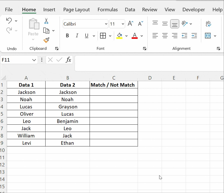
Example using IF condition to show “Match” or “Not a Match”:

In cell C2, enter the formula =IF(A2=B2,"Match","Not a Match") and drag it down.

This method provides a more user-friendly output compared to TRUE/FALSE and enhances readability, especially in larger datasets.

3. EXACT Function: Case-Sensitive Comparison

In most cases, Excel comparisons are case-insensitive, meaning “Apple” and “apple” are treated as the same. However, if you need a case-sensitive comparison, the EXACT function is the solution. EXACT compares two text strings and returns TRUE only if they are exactly the same, including case.

Formula:

=EXACT(text1, text2)

How to use it for column comparison:

In cell C2, enter the formula =IF(EXACT(A2, B2), "Match", "Mismatch") and drag it down.
The EXACT(A2, B2) part performs a case-sensitive comparison between cells A2 and B2.
The IF function then displays “Match” if EXACT returns TRUE (case-sensitive match) and “Mismatch” if it returns FALSE.

Example:

If cell A2 contains “Excel” and cell B2 contains “excel”, using =A2=B2 would return “Match” (TRUE), while =IF(EXACT(A2, B2), "Match", "Mismatch") would return “Mismatch” (FALSE) because of the case difference.

The EXACT function is crucial when case sensitivity is important for your data comparison, such as when dealing with usernames, codes, or product identifiers where case variations matter.

4. Conditional Formatting: Visually Highlight Differences and Duplicates

Conditional formatting offers a powerful way to visually highlight matching, duplicate, or unique values directly within your columns, without needing an extra column for results. This method is excellent for quickly identifying patterns and anomalies within your data.

Highlighting Duplicate Values (Values present in both columns):

Select both columns of data you want to compare (e.g., columns A and B).
Go to the Home tab on the Excel ribbon.
In the Styles group, click Conditional Formatting.
Select Highlight Cells Rules and then Duplicate Values….
In the “Duplicate Values” dialog box:
- Ensure “Duplicate” is selected in the dropdown.
- Choose your desired formatting style (e.g., fill color, text color, border).
- Click OK.

Excel will now highlight all values that appear in both selected columns, making it easy to visually spot common entries.

Highlighting Unique Values (Values present in only one of the columns):

Follow steps 1-3 above.
In the “Highlight Cells Rules” menu, select Duplicate Values….
In the “Duplicate Values” dialog box:
- Change the dropdown from “Duplicate” to Unique.
- Choose your desired formatting style.
- Click OK.

Excel will now highlight values that are unique, meaning they appear in one column but not the other. This is helpful for identifying entries that are exclusive to each list.

Customizing Conditional Formatting:

Excel offers various formatting options in the “Duplicate Values” dialog, including predefined styles and the “Custom Format” option, which allows you to create your own formatting rules using fill colors, fonts, borders, and more.

Clearing Conditional Formatting:

To remove conditional formatting, select the formatted cells, go to Conditional Formatting, then Clear Rules, and choose Clear Rules from Selected Cells.

Example of Conditional Formatting for Duplicate Values:

Example of Conditional Formatting for Unique Values:

Conditional formatting is a visually intuitive and dynamic way to compare columns, especially for smaller to medium-sized datasets where visual identification of patterns is beneficial.

5. VLOOKUP Function: Finding Matches and Missing Values

The VLOOKUP function is a powerful lookup and reference function that can also be effectively used to compare columns, particularly when you need to determine if values from one column exist in another. VLOOKUP searches for a value in the first column of a table and returns a corresponding value from a specified column in the same row.

Formula:

=VLOOKUP(lookup_value, table_array, col_index_num, [range_lookup])

How to use VLOOKUP for column comparison:

Let’s say you have a list of items in column A (lookup column) and another list in column B (comparison column). You want to check for each item in column A if it is present in column B.

In cell C2 (or any empty column), enter the formula =VLOOKUP(A2, $B$2:$B$5, 1, FALSE). (Note: Adjust the range $B$2:$B$5 to cover the entire range of your comparison column B. The $ signs create absolute references, ensuring the range doesn’t change when you drag the formula down.)
Drag the fill handle down to apply the formula to all rows in column A.

Understanding the formula:

A2: This is the lookup_value – the value from column A that you want to search for in column B.
$B$2:$B$5: This is the table_array – the range of cells in column B where VLOOKUP will search for the lookup_value.
1: This is the col_index_num – it specifies which column in the table_array to return a value from. Since we are just checking for existence, we can use 1 (the first column of the table_array, which is column B itself).
FALSE: This is the range_lookup argument. FALSE (or 0) ensures that VLOOKUP only finds exact matches.

Interpreting the results:

If VLOOKUP finds a match for the value from column A in column B, it will return the matching value from column B in column C.
If VLOOKUP does not find a match, it will return #N/A in column C, indicating that the value from column A is not present in column B.

Example using VLOOKUP to compare exam subjects:

VLOOKUP is particularly useful for comparing one column against another to identify missing values or confirm the presence of specific entries. While it can seem more complex than simpler methods, it offers significant power and flexibility for more sophisticated column comparisons.

Frequently Asked Questions

1. How to quickly compare two columns in Excel for differences using “Go To Special”?

Excel’s “Go To Special” feature provides a rapid way to highlight row differences between two columns.

Steps:

Select both columns you want to compare.
Press Ctrl + G (or F5) to open the “Go To” dialog box.
Click Special….
In the “Go To Special” dialog box, select Row differences.
Click OK.

Excel will select the cells that are different row-by-row between the two columns. The unmatched cells will appear visually distinct (often with a gray background compared to white for matching cells, depending on your Excel theme). This is a quick visual check for differences without formulas.

2. What are other methods to compare more than two columns in Excel using the IF condition?

While the basic IF condition compares two columns, you can extend it to compare multiple columns using logical functions like AND and OR.

To find rows where values in ALL compared columns are the same: Use the AND function within the IF condition. For example, to check if columns A, B, and C have matching values in each row, use the formula: =IF(AND(A2=B2, A2=C2), "Full Match", ""). This will return “Full Match” only if A2=B2 AND A2=C2.
To find rows where values in ANY of the compared columns match: Use the OR function within the IF condition. For example, to check if there’s a match between any pair of values in columns A, B, and C, use: =IF(OR(A2=B2, B2=C2, A2=C2), "Match", ""). This will return “Match” if A2=B2 OR B2=C2 OR A2=C2.

These combined formulas allow you to perform more complex multi-column comparisons using the IF function.

3. Can you compare two columns in Excel using the INDEX-MATCH function?

Yes, INDEX-MATCH is another powerful lookup combination that can be used for column comparison, often offering more flexibility than VLOOKUP, especially when dealing with more complex data structures.

Example using INDEX-MATCH for column comparison:

Suppose you have a list of IDs in column D and want to check if these IDs exist in column A, and if so, retrieve the corresponding Name from column B.

In cell E2, you can use the formula: =IFERROR(INDEX($B$2:$B$4, MATCH(D2, $A$2:$A$4, 0)), "#N/A").

Explanation:

MATCH(D2, $A$2:$A$4, 0): This part searches for the value in D2 within the range A2:A4 (column A) and returns the relative position of the match. 0 specifies an exact match.
INDEX($B$2:$B$4, ...): The INDEX function then uses the position returned by MATCH to retrieve the corresponding value from the range B2:B4 (column B).
IFERROR(..., "#N/A"): This handles cases where MATCH doesn’t find a match (ID from column D not in column A), and returns “#N/A” instead of an error.

INDEX-MATCH provides a flexible alternative to VLOOKUP for column comparison, particularly when you need to retrieve corresponding values based on matches and handle potential errors gracefully.

Conclusion

Comparing two columns in Excel is a fundamental skill for anyone working with data. This guide has explored a range of methods, from simple operators and IF conditions to conditional formatting and lookup functions like VLOOKUP and INDEX-MATCH. Each technique offers unique advantages and is suited to different comparison scenarios.

By mastering these techniques, you can significantly enhance your efficiency and accuracy in data analysis. Whether you need to identify duplicates, highlight differences, or validate data across columns, Excel provides the tools to streamline your workflow and unlock valuable insights from your spreadsheets. Continue to explore Excel’s vast capabilities to further refine your data handling skills and become a proficient data analyst. Consider delving deeper into advanced Excel courses to expand your knowledge of functions, formulas, and data analysis techniques.