How To Compare Two Columns In Different Excel Workbooks

COMPARE.EDU.VN presents a comprehensive guide on How To Compare Two Columns In Different Excel Workbooks, offering a streamlined solution for data analysis and validation. This article provides detailed methods and techniques to effectively compare data across multiple Excel files, ensuring accuracy and efficiency. Unlock the power of cross-workbook comparison, data matching, and discrepancy identification to make informed decisions and maintain data integrity using lookup functions and conditional formatting.

1. Understanding the Need for Cross-Workbook Column Comparison

Comparing columns across different Excel workbooks is a common task in various professional scenarios. Whether you’re merging data from multiple sources, validating data integrity, or identifying discrepancies between datasets, the ability to efficiently compare columns is essential. This process involves matching data from one workbook to another and highlighting any differences or similarities. Let’s explore why this is crucial and the potential challenges involved.

1.1. Scenarios Requiring Column Comparison

Several situations necessitate comparing columns in different Excel workbooks:

• Data Consolidation: When merging data from multiple Excel files into a single master sheet, you need to ensure data consistency and accuracy by comparing columns to identify duplicates or inconsistencies.
• Data Validation: Validating data integrity across different systems or databases often involves comparing columns in Excel to verify that the data matches as expected.
• Financial Analysis: Financial analysts frequently compare columns in different workbooks to track financial performance, analyze trends, and identify discrepancies between budgets and actuals.
• Inventory Management: Comparing inventory lists across different Excel files helps identify stock discrepancies, track product movements, and ensure accurate inventory levels.
• Sales Reporting: Comparing sales data from different regions or time periods requires comparing columns in separate workbooks to identify top-performing products, sales trends, and areas for improvement.

1.2. Challenges in Comparing Columns

Despite its importance, comparing columns in different Excel workbooks can present several challenges:

• Large Datasets: Working with large datasets can make manual comparison time-consuming and prone to errors.
• Data Inconsistencies: Variations in data formatting, spelling errors, and inconsistencies in data entry can complicate the comparison process.
• Workbook Complexity: Complex workbooks with multiple sheets and formulas can make it difficult to locate and compare the relevant columns.
• Time Constraints: Tight deadlines and the need for quick insights often require efficient methods for comparing columns without sacrificing accuracy.
• Error Prone: Manual comparison is highly susceptible to human error, especially when dealing with large and complex datasets.

2. Essential Excel Functions for Column Comparison

Excel offers several built-in functions that can significantly simplify the process of comparing columns in different workbooks. These functions allow you to automate the comparison, identify matches and differences, and extract relevant data based on your criteria. Here’s an overview of some essential Excel functions for column comparison.

2.1. VLOOKUP for Finding Matches

VLOOKUP (Vertical Lookup) is a powerful Excel function used to search for a value in the first column of a range and return a value in the same row from another column in the range. It is particularly useful for comparing columns in different workbooks to find matches and retrieve corresponding data.

Syntax:

VLOOKUP(lookup_value, table_array, col_index_num, [range_lookup])

• lookup_value: The value you want to search for in the first column of the table array.
• table_array: The range of cells that contains the data you want to search in.
• col_index_num: The column number in the table array from which you want to return a value.
• [range_lookup]: Optional. A logical value that specifies whether you want VLOOKUP to find an exact or approximate match. TRUE or omitted finds an approximate match; FALSE finds an exact match.

Example:

Suppose you have two Excel workbooks: “SalesData_2022.xlsx” and “SalesData_2023.xlsx”. Both workbooks contain a “Sales” sheet with a “ProductID” column and a “ProductName” column. You want to compare the “ProductID” column in “SalesData_2022.xlsx” with the “ProductID” column in “SalesData_2023.xlsx” and retrieve the corresponding “ProductName” from “SalesData_2023.xlsx”.

1. Open “SalesData_2022.xlsx” and select the cell where you want to display the “ProductName” (e.g., cell C2).
2. Enter the following formula:

=VLOOKUP(A2,'[SalesData_2023.xlsx]Sales'!A:B,2,FALSE)

• A2: The “ProductID” in “SalesData_2022.xlsx” that you want to search for.
• '[SalesData_2023.xlsx]Sales'!A:B: The range of cells in “SalesData_2023.xlsx” that contains the “ProductID” and “ProductName” columns.
• 2: The column number in the table array from which you want to return a value (i.e., the “ProductName” column).
• FALSE: Specifies that you want VLOOKUP to find an exact match.

3. Press Enter to apply the formula. Excel will search for the “ProductID” in “SalesData_2023.xlsx” and return the corresponding “ProductName” in cell C2.
4. Drag the fill handle (the small square at the bottom right corner of the cell) down to apply the formula to the remaining cells in column C.

2.2. MATCH for Identifying Row Numbers

The MATCH function in Excel is used to find the position of a specified value within a range of cells. It returns the relative position of the matched item in the range. This function is particularly useful when you need to identify the row number of a specific value in a column.

Syntax:

MATCH(lookup_value, lookup_array, [match_type])

• lookup_value: The value you want to find in the lookup array.
• lookup_array: The range of cells you want to search in.
• [match_type]: Optional. Specifies how MATCH should match the lookup value with the values in the lookup array.
  • 0: Finds the first value that is exactly equal to the lookup value.
  • 1: Finds the largest value that is less than or equal to the lookup value. The lookup array must be sorted in ascending order.
  • -1: Finds the smallest value that is greater than or equal to the lookup value. The lookup array must be sorted in descending order.

Example:

Suppose you have two Excel workbooks: “EmployeeData_2022.xlsx” and “EmployeeData_2023.xlsx”. Both workbooks contain an “Employees” sheet with an “EmployeeID” column. You want to find the row number of a specific “EmployeeID” in the “EmployeeID” column of “EmployeeData_2023.xlsx”.

1. Open “EmployeeData_2022.xlsx” and select the cell where you want to display the row number (e.g., cell B2).
2. Enter the following formula:

=MATCH(A2,'[EmployeeData_2023.xlsx]Employees'!A:A,0)

• A2: The “EmployeeID” in “EmployeeData_2022.xlsx” that you want to search for.
• '[EmployeeData_2023.xlsx]Employees'!A:A: The range of cells in “EmployeeData_2023.xlsx” that contains the “EmployeeID” column.
• 0: Specifies that you want MATCH to find an exact match.

3. Press Enter to apply the formula. Excel will search for the “EmployeeID” in “EmployeeData_2023.xlsx” and return the row number where the “EmployeeID” is found.
4. Drag the fill handle down to apply the formula to the remaining cells in column B.

2.3. INDEX for Retrieving Data

The INDEX function in Excel is used to return a value or the reference to a value from within a range or array. It is a versatile function that can be used in combination with other functions, such as MATCH, to retrieve data from specific locations in a worksheet.

Syntax:

INDEX(array, row_num, [column_num])

• array: The range of cells from which you want to return a value.
• row_num: The row number in the array from which you want to return a value.
• [column_num]: Optional. The column number in the array from which you want to return a value. If omitted, column_num is assumed to be 1.

Example:

Suppose you have two Excel workbooks: “ProductList_2022.xlsx” and “ProductList_2023.xlsx”. Both workbooks contain a “Products” sheet with a “ProductID” column and a “ProductName” column. You want to retrieve the “ProductName” from “ProductList_2023.xlsx” based on the “ProductID” in “ProductList_2022.xlsx”.

1. Open “ProductList_2022.xlsx” and select the cell where you want to display the “ProductName” (e.g., cell C2).
2. Enter the following formula:

=INDEX('[ProductList_2023.xlsx]Products'!B:B,MATCH(A2,'[ProductList_2023.xlsx]Products'!A:A,0))

• '[ProductList_2023.xlsx]Products'!B:B: The range of cells in “ProductList_2023.xlsx” that contains the “ProductName” column.
• MATCH(A2,'[ProductList_2023.xlsx]Products'!A:A,0): The MATCH function finds the row number of the “ProductID” in “ProductList_2023.xlsx”.
• A2: The “ProductID” in “ProductList_2022.xlsx” that you want to search for.
• '[ProductList_2023.xlsx]Products'!A:A: The range of cells in “ProductList_2023.xlsx” that contains the “ProductID” column.
• 0: Specifies that you want MATCH to find an exact match.

3. Press Enter to apply the formula. Excel will search for the “ProductID” in “ProductList_2023.xlsx” and return the corresponding “ProductName” in cell C2.
4. Drag the fill handle down to apply the formula to the remaining cells in column C.

2.4. IF for Conditional Checks

The IF function in Excel is a logical function that returns one value if a condition is true and another value if the condition is false. It is useful for performing conditional checks and making decisions based on the comparison of values.

Syntax:

IF(logical_test, value_if_true, value_if_false)

• logical_test: The condition you want to evaluate.
• value_if_true: The value to return if the condition is true.
• value_if_false: The value to return if the condition is false.

Example:

Suppose you have two Excel workbooks: “OrderData_2022.xlsx” and “OrderData_2023.xlsx”. Both workbooks contain an “Orders” sheet with an “OrderID” column and an “OrderAmount” column. You want to compare the “OrderAmount” for the same “OrderID” in both workbooks and display “Match” if the amounts are the same and “Mismatch” if they are different.

1. Open “OrderData_2022.xlsx” and select the cell where you want to display the result (e.g., cell C2).
2. Enter the following formula:

=IF(B2='[OrderData_2023.xlsx]Orders'!B2,"Match","Mismatch")

• B2: The “OrderAmount” in “OrderData_2022.xlsx” that you want to compare.
• '[OrderData_2023.xlsx]Orders'!B2: The corresponding “OrderAmount” in “OrderData_2023.xlsx”.
• "Match": The value to return if the “OrderAmount”s are the same.
• "Mismatch": The value to return if the “OrderAmount”s are different.

3. Press Enter to apply the formula. Excel will compare the “OrderAmount”s and display “Match” or “Mismatch” in cell C2.
4. Drag the fill handle down to apply the formula to the remaining cells in column C.

2.5. COUNTIF for Counting Occurrences

The COUNTIF function in Excel is used to count the number of cells within a range that meet a given criterion. It is useful for determining how many times a specific value appears in a column.

Syntax:

COUNTIF(range, criteria)

• range: The range of cells you want to count.
• criteria: The condition or value you want to count.

Example:

Suppose you have two Excel workbooks: “CustomerList_2022.xlsx” and “CustomerList_2023.xlsx”. Both workbooks contain a “Customers” sheet with a “CustomerID” column. You want to count how many times each “CustomerID” in “CustomerList_2022.xlsx” appears in the “CustomerID” column of “CustomerList_2023.xlsx”.

1. Open “CustomerList_2022.xlsx” and select the cell where you want to display the count (e.g., cell C2).
2. Enter the following formula:

=COUNTIF('[CustomerList_2023.xlsx]Customers'!A:A,A2)

• '[CustomerList_2023.xlsx]Customers'!A:A: The range of cells in “CustomerList_2023.xlsx” that contains the “CustomerID” column.
• A2: The “CustomerID” in “CustomerList_2022.xlsx” that you want to count.

3. Press Enter to apply the formula. Excel will count how many times the “CustomerID” appears in “CustomerList_2023.xlsx” and display the count in cell C2.
4. Drag the fill handle down to apply the formula to the remaining cells in column C.

3. Step-by-Step Guide to Comparing Two Columns

Here’s a step-by-step guide to comparing two columns in different Excel workbooks, incorporating the functions and techniques discussed above.

3.1. Preparing the Data

Before you start comparing columns, it’s important to prepare your data to ensure accurate and efficient results.

1. Open Both Workbooks: Open the two Excel workbooks you want to compare.
2. Identify Columns to Compare: Determine which columns in each workbook you want to compare. Make sure the columns contain similar data types (e.g., text, numbers, dates).
3. Clean the Data: Clean the data in both columns to remove any inconsistencies or errors. This may involve:
   • Removing leading or trailing spaces
   • Correcting spelling errors
   • Standardizing data formats (e.g., dates, phone numbers)
   • Removing duplicate entries
4. Sort the Data (Optional): Sorting the data in both columns can make it easier to identify matches and differences. Sort both columns in the same order (e.g., ascending or descending).

3.2. Using VLOOKUP for Comparison

VLOOKUP is a versatile function for comparing columns and retrieving corresponding data.

1. Open the First Workbook: Open the Excel workbook where you want to display the comparison results.
2. Select a Cell: Select the cell where you want to display the result of the comparison (e.g., cell C2).
3. Enter the VLOOKUP Formula: Enter the VLOOKUP formula to compare the columns in the two workbooks.

=VLOOKUP(A2,'[Workbook2.xlsx]Sheet1'!A:B,2,FALSE)

• A2: The value in the first workbook that you want to search for in the second workbook.
• '[Workbook2.xlsx]Sheet1'!A:B: The range of cells in the second workbook that contains the data you want to search in.
• 2: The column number in the table array from which you want to return a value.
• FALSE: Specifies that you want VLOOKUP to find an exact match.

4. Apply the Formula: Press Enter to apply the formula. Excel will search for the value in the first workbook and return the corresponding value from the second workbook.
5. Drag the Fill Handle: Drag the fill handle down to apply the formula to the remaining cells in the column.

3.3. Using IF for Conditional Checks

The IF function is useful for performing conditional checks and highlighting matches and differences.

1. Open the First Workbook: Open the Excel workbook where you want to display the comparison results.
2. Select a Cell: Select the cell where you want to display the result of the comparison (e.g., cell C2).
3. Enter the IF Formula: Enter the IF formula to compare the columns in the two workbooks.

=IF(B2='[Workbook2.xlsx]Sheet1'!B2,"Match","Mismatch")

• B2: The value in the first workbook that you want to compare.
• '[Workbook2.xlsx]Sheet1'!B2: The corresponding value in the second workbook.
• "Match": The value to return if the values are the same.
• "Mismatch": The value to return if the values are different.

4. Apply the Formula: Press Enter to apply the formula. Excel will compare the values and display “Match” or “Mismatch” in the cell.
5. Drag the Fill Handle: Drag the fill handle down to apply the formula to the remaining cells in the column.

3.4. Identifying Differences Using Conditional Formatting

Conditional formatting can be used to automatically highlight differences between columns.

1. Select the Column: Select the column in the first workbook that you want to compare.
2. Open Conditional Formatting: Go to the “Home” tab in the Excel ribbon and click on “Conditional Formatting”.
3. New Rule: Select “New Rule” from the dropdown menu.
4. Use a Formula: Choose “Use a formula to determine which cells to format”.
5. Enter the Formula: Enter the formula to compare the columns in the two workbooks.

=B2<>'[Workbook2.xlsx]Sheet1'!B2

• B2: The value in the first workbook that you want to compare.
• '[Workbook2.xlsx]Sheet1'!B2: The corresponding value in the second workbook.

6. Format: Click on the “Format” button to choose a formatting style (e.g., fill color, font color) to highlight the differences.
7. Apply the Rule: Click “OK” to apply the conditional formatting rule. Excel will automatically highlight the cells in the column that are different from the corresponding cells in the second workbook.

4. Advanced Techniques and Tips

To enhance your column comparison skills, consider these advanced techniques and tips.

4.1. Using Array Formulas

Array formulas can perform calculations on multiple values at once, making them useful for complex comparisons.

Example:

To compare two columns and return an array of “Match” or “Mismatch” results:

1. Select a Range: Select a range of cells where you want to display the results.
2. Enter the Array Formula: Enter the following array formula:

=IF(A1:A10= '[Workbook2.xlsx]Sheet1'!A1:A10,"Match","Mismatch")

3. Press Ctrl+Shift+Enter: Press Ctrl+Shift+Enter to enter the formula as an array formula. Excel will display the results in the selected range.

4.2. Combining Functions for Complex Logic

You can combine multiple Excel functions to create complex comparison logic.

Example:

To compare two columns and check if both the “ProductID” and “ProductName” match:

=IF(AND(A2='[Workbook2.xlsx]Sheet1'!A2,B2='[Workbook2.xlsx]Sheet1'!B2),"Match","Mismatch")

4.3. Handling Errors and Missing Data

When comparing columns, it’s important to handle errors and missing data gracefully.

Example:

To handle errors when using VLOOKUP, use the IFERROR function:

=IFERROR(VLOOKUP(A2,'[Workbook2.xlsx]Sheet1'!A:B,2,FALSE),"Not Found")

4.4. Automating the Process with Macros

For repetitive tasks, you can automate the column comparison process using Excel macros.

1. Open VBA Editor: Press Alt + F11 to open the Visual Basic Editor (VBE).
2. Insert a Module: In the VBE, go to “Insert” > “Module”.
3. Write the Macro: Write a macro to compare the columns and perform the desired actions.

Sub CompareColumns()
    Dim wb1 As Workbook, wb2 As Workbook
    Dim ws1 As Worksheet, ws2 As Worksheet
    Dim LastRow As Long, i As Long

    'Set the workbooks and worksheets
    Set wb1 = ThisWorkbook
    Set ws1 = wb1.Sheets("Sheet1")
    Set wb2 = Workbooks.Open("C:PathToYourWorkbook2.xlsx")
    Set ws2 = wb2.Sheets("Sheet1")

    'Get the last row in the first worksheet
    LastRow = ws1.Cells(Rows.Count, "A").End(xlUp).Row

    'Loop through the rows and compare the columns
    For i = 2 To LastRow
        If ws1.Cells(i, "B").Value = ws2.Cells(i, "B").Value Then
            ws1.Cells(i, "C").Value = "Match"
        Else
            ws1.Cells(i, "C").Value = "Mismatch"
        End If
    Next i

    'Close the second workbook
    wb2.Close SaveChanges:=False

    MsgBox "Column comparison complete!"
End Sub

4. Run the Macro: Run the macro to automate the column comparison process.

5. Real-World Examples and Case Studies

Let’s examine some real-world examples and case studies to illustrate the practical applications of comparing columns in different Excel workbooks.

5.1. Financial Data Reconciliation

A financial analyst needs to reconcile financial data from two different systems. One system contains the general ledger data, while the other contains the accounts receivable data. The analyst needs to compare the transaction amounts for each account to identify any discrepancies.

Solution:

1. Export Data: Export the data from both systems into Excel workbooks.
2. Clean Data: Clean the data to ensure consistency in data formats and remove any errors.
3. Use VLOOKUP: Use VLOOKUP to compare the transaction amounts for each account in the two workbooks.
4. Use IF: Use the IF function to flag any discrepancies between the transaction amounts.
5. Conditional Formatting: Use conditional formatting to highlight the discrepancies for further investigation.

5.2. Inventory Management

An inventory manager needs to compare the inventory levels in two different warehouses. Each warehouse maintains its own Excel file with the inventory data. The manager needs to identify any discrepancies in the inventory levels to ensure accurate stock management.

Solution:

1. Open Workbooks: Open the Excel workbooks for both warehouses.
2. Identify Columns: Identify the columns containing the product ID and the inventory levels.
3. Use VLOOKUP: Use VLOOKUP to compare the inventory levels for each product in the two warehouses.
4. Use IF: Use the IF function to flag any discrepancies between the inventory levels.
5. Calculate Variance: Calculate the variance between the inventory levels to quantify the discrepancies.

5.3. Sales Data Analysis

A sales manager needs to compare the sales data from two different regions. Each region maintains its own Excel file with the sales data. The manager needs to identify the top-performing products in each region and compare their sales performance.

Solution:

1. Open Workbooks: Open the Excel workbooks for both regions.
2. Identify Columns: Identify the columns containing the product ID, product name, and sales amount.
3. Use VLOOKUP: Use VLOOKUP to compare the sales amounts for each product in the two regions.
4. Sort Data: Sort the data by sales amount to identify the top-performing products in each region.
5. Create Charts: Create charts to visualize the sales performance of the top-performing products in each region.

6. Common Mistakes to Avoid

When comparing columns in different Excel workbooks, it’s important to avoid common mistakes that can lead to inaccurate results.

6.1. Incorrect Formula Syntax

Ensure that you use the correct syntax for Excel functions such as VLOOKUP, MATCH, INDEX, and IF. Double-check the arguments and make sure they are in the correct order.

6.2. Not Handling Errors

Use the IFERROR function to handle errors that may occur when comparing columns, such as when a value is not found in the lookup range.

6.3. Ignoring Data Types

Make sure that the data types in the columns you are comparing are consistent. Comparing text values with numeric values can lead to unexpected results.

6.4. Overlooking Case Sensitivity

Excel is case-insensitive by default. If you need to perform a case-sensitive comparison, use the EXACT function.

6.5. Forgetting Absolute References

Use absolute references ($) to prevent the lookup range from changing when you drag the fill handle.

7. Optimize Your Workflow with COMPARE.EDU.VN

Comparing columns in different Excel workbooks can be a complex and time-consuming task. However, by using the right techniques and tools, you can streamline the process and ensure accurate results. COMPARE.EDU.VN offers a variety of resources and tools to help you optimize your workflow and make informed decisions.

7.1. Find the Best Tools

COMPARE.EDU.VN provides comprehensive reviews and comparisons of various Excel add-ins and tools that can simplify the process of comparing columns in different workbooks. Our expert reviews help you find the tools that best meet your specific needs and budget.

7.2. Access Expert Guides

Our website offers a wealth of expert guides and tutorials that cover a wide range of Excel topics, including column comparison techniques. Whether you’re a beginner or an experienced Excel user, you’ll find valuable insights and tips to improve your skills.

7.3. Compare Different Approaches

COMPARE.EDU.VN allows you to compare different approaches to column comparison and choose the method that is most efficient and effective for your specific scenario. Our detailed comparisons highlight the pros and cons of each approach, helping you make informed decisions.

8. Call to Action

Ready to streamline your column comparison process and make informed decisions? Visit COMPARE.EDU.VN today to find the best tools, access expert guides, and compare different approaches. Simplify your data analysis and ensure accurate results with our comprehensive resources.

For further assistance or inquiries, please contact us at:

• Address: 333 Comparison Plaza, Choice City, CA 90210, United States
• Whatsapp: +1 (626) 555-9090
• Website: compare.edu.vn

9. FAQs About Comparing Columns in Excel

9.1. Can I compare more than two columns at once?

Yes, you can compare more than two columns at once by nesting multiple IF functions or using array formulas. However, keep in mind that complex formulas can be more difficult to understand and maintain.

9.2. How do I compare columns with different lengths?

When comparing columns with different lengths, you can use the IFERROR function to handle the case where a value is not found in the lookup range. Alternatively, you can use the MATCH function to identify the last row with data in each column and adjust the comparison range accordingly.

9.3. Can I compare columns in different Excel versions?

Yes, you can compare columns in different Excel versions as long as the Excel files are compatible. However, keep in mind that some features and functions may not be available in older versions of Excel.

9.4. How do I compare columns with case-sensitive data?

Excel is case-insensitive by default. To perform a case-sensitive comparison, use the EXACT function. The EXACT function compares two text strings and returns TRUE if they are exactly the same, including case.

9.5. Can I compare columns with special characters?

Yes, you can compare columns with special characters as long as the characters are properly encoded and recognized by Excel. However, keep in mind that some special characters may have different meanings in different Excel versions or regional settings.

9.6. How do I compare columns with dates?

When comparing columns with dates, make sure that the dates are formatted consistently. You can use the TEXT function to format the dates before comparing them.

9.7. Can I automate the column comparison process?

Yes, you can automate the column comparison process using Excel macros. Macros allow you to write custom code to perform repetitive tasks and automate complex workflows.

9.8. How do I handle errors when comparing columns?

Use the IFERROR function to handle errors that may occur when comparing columns, such as when a value is not found in the lookup range. The IFERROR function allows you to specify a value to return if an error occurs.

9.9. Can I use conditional formatting to highlight differences between columns?

Yes, you can use conditional formatting to automatically highlight differences between columns. Conditional formatting allows you to apply formatting rules to cells based on their values or formulas.

9.10. What are the best practices for comparing columns in Excel?

Some best practices for comparing columns in Excel include:

• Preparing the data to ensure consistency and accuracy.
• Using the correct Excel functions for the comparison task.
• Handling errors and missing data gracefully.
• Automating the process with macros for repetitive tasks.
• Validating the results to ensure accuracy.
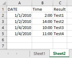  Example Excel sheet

By following these best practices, you can streamline your column comparison process and make informed decisions based on accurate data.