Comparing two columns from different sheets in Excel can be a complex task. If you are looking for a reliable solution to streamline your data comparison tasks, COMPARE.EDU.VN offers comprehensive guides and tools to help you efficiently compare data. Discover practical techniques and step-by-step instructions on how to achieve accurate comparisons between your Excel sheets. Leverage the power of Excel to analyze, match, and reconcile data across different worksheets with ease using robust methods for data validation, conditional formatting, and formula-based comparisons.
1. Understanding the Need for Cross-Sheet Column Comparison in Excel
When working with large datasets in Excel, it is often necessary to compare data residing in different sheets. This task is crucial for data validation, identifying discrepancies, and ensuring data integrity. Understanding why you need to compare columns across sheets is the first step toward choosing the right technique. Whether you’re merging data, auditing records, or simply looking for differences, knowing your objective will guide your approach. COMPARE.EDU.VN offers resources that delve into common data comparison scenarios, providing context and helping users frame their specific needs.
1.1. Common Scenarios Requiring Column Comparison
Data professionals frequently encounter situations where column comparison across different Excel sheets becomes essential. One typical scenario involves merging customer databases from separate regional offices to create a unified customer view. Each sheet might contain customer IDs, names, and contact details, and comparing columns such as customer IDs is necessary to identify duplicates and ensure data consistency. Another common use case arises in financial auditing. Auditors often need to compare transaction records from different accounting periods or sources to detect discrepancies or inconsistencies. This might involve comparing columns for transaction dates, amounts, and descriptions to ensure accuracy and compliance.
Supply chain management also benefits significantly from cross-sheet column comparison. Supply chain analysts often work with data from multiple suppliers, each providing information in separate sheets. Comparing columns such as product codes, order quantities, and delivery dates is crucial for tracking inventory levels, managing orders, and identifying potential bottlenecks. In scientific research, researchers may need to compare data from multiple experiments or data sources, each stored in separate sheets. Comparing columns such as sample IDs, measurements, and experimental conditions is necessary to validate results and draw meaningful conclusions. These scenarios highlight the diverse and critical applications of comparing columns across different Excel sheets in various professional fields.
1.2. Benefits of Efficient Data Comparison
Efficiently comparing data between columns from different sheets offers numerous benefits that can significantly enhance productivity and accuracy. One of the primary advantages is the ability to identify discrepancies quickly and accurately. By automating the comparison process, you can detect inconsistencies, errors, and outliers that might otherwise go unnoticed. This is particularly valuable in financial analysis, where even small errors can have significant consequences. Another key benefit is improved data quality. Regularly comparing and reconciling data across different sheets helps ensure that your datasets are accurate, consistent, and reliable. This, in turn, leads to better decision-making and more trustworthy insights.
Efficient data comparison also saves considerable time and effort. Manually comparing large datasets is time-consuming and prone to human error. By using Excel functions and tools, you can automate the comparison process, freeing up time for more strategic tasks. Furthermore, efficient data comparison facilitates better data integration. When merging data from multiple sources, it’s essential to identify and resolve any conflicts or inconsistencies. Comparing columns across different sheets allows you to seamlessly integrate data while maintaining data integrity. Overall, efficient data comparison not only enhances accuracy and saves time but also promotes better data management and informed decision-making.
2. Preparing Your Excel Sheets for Comparison
Before diving into the technical aspects of comparing columns, proper preparation of your Excel sheets is vital. This involves ensuring consistency in data formatting, handling missing values, and understanding the size and structure of your datasets. Poor preparation can lead to inaccurate results and wasted effort. COMPARE.EDU.VN emphasizes the importance of cleaning and organizing your data before attempting any comparison, highlighting common pitfalls and providing practical solutions.
2.1. Ensuring Data Consistency
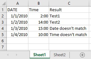
Data consistency is paramount when comparing columns from different Excel sheets. Inconsistencies in data format can lead to inaccurate comparison results, even if the underlying data is the same. One common issue is inconsistent date formats. For example, one sheet might use “MM/DD/YYYY” while another uses “DD/MM/YYYY”. Before comparing date columns, ensure they are formatted identically. Excel provides several date formatting options under the “Format Cells” menu, accessible by right-clicking on the column header and selecting “Format Cells”. Choose a standard date format that is consistent across all sheets. Another frequent inconsistency arises with text case. For instance, one sheet might use “Apple” while another uses “apple”. Excel’s UPPER(), LOWER(), and PROPER() functions can help standardize text case.
To convert all text in a column to uppercase, use the formula =UPPER(A1) in a new column, where A1 is the first cell in the text column. Similarly, you can use =LOWER(A1) for lowercase and =PROPER(A1) to capitalize the first letter of each word. Leading or trailing spaces can also cause comparison issues. Use the TRIM() function to remove these spaces. For example, if cell A1 contains text with leading or trailing spaces, the formula =TRIM(A1) will remove those spaces. Numeric inconsistencies, such as differences in decimal places or currency symbols, can also skew comparison results. Ensure that numbers are formatted consistently using the “Format Cells” menu. Specify the number of decimal places and choose the appropriate currency symbol, if applicable. Addressing these common inconsistencies ensures that your data is uniform and ready for accurate comparison.
2.2. Handling Missing Values and Errors
Missing values and errors can significantly impact the accuracy of column comparisons in Excel. It’s crucial to address these issues before proceeding with any comparison techniques. One common approach to handling missing values is to replace them with a standardized value, such as “N/A” or “0”, depending on the context of the data. Excel’s IFERROR() function can be used to replace errors with a specified value. For example, if cell A1 contains a formula that might result in an error, you can use the formula =IFERROR(A1, "Error") to replace any errors with the text “Error”. Another strategy is to filter out rows containing missing values or errors.
Excel’s filtering feature allows you to quickly identify and exclude rows with specific values or errors. To use filtering, select the column header and click on the “Filter” button in the “Data” tab. Then, you can filter out rows containing blank cells, errors, or other unwanted values. In some cases, it might be appropriate to impute missing values based on statistical methods. For example, you could replace missing values with the mean, median, or mode of the column. Excel’s AVERAGE(), MEDIAN(), and MODE() functions can be used to calculate these values. However, imputation should be used cautiously, as it can introduce bias into your data. It’s also important to document how missing values and errors were handled to maintain transparency and ensure the validity of your analysis. By addressing these issues proactively, you can minimize the impact of missing values and errors on your column comparisons and ensure more accurate results.
2.3. Understanding Data Size and Structure
The size and structure of your data play a crucial role in determining the most efficient comparison method. Large datasets may require more advanced techniques or tools to avoid performance issues, while smaller datasets can be easily managed with simple formulas. Understanding the number of rows and columns in each sheet helps you anticipate potential challenges and plan your approach accordingly. You can quickly determine the size of your data by selecting the entire dataset and looking at the row and column counts in the bottom-right corner of the Excel window. The structure of your data, including the presence of headers, unique identifiers, and data types, also influences your comparison strategy. Ensure that both sheets have consistent header names for the columns you intend to compare.
If the data structures are significantly different, you may need to reshape the data before performing the comparison. This might involve transposing rows and columns, merging or splitting columns, or using lookup functions to align data. COMPARE.EDU.VN provides guidance on data transformation techniques to help you standardize your data structure. Furthermore, consider whether your data is sorted or unsorted. Sorted data can often be compared more efficiently using techniques such as binary search or sequential comparison. Unsorted data may require more complex algorithms to ensure accurate matching. By carefully assessing the size and structure of your data, you can select the most appropriate comparison method and optimize your workflow for efficiency and accuracy.
3. Basic Excel Functions for Column Comparison
Excel offers a range of built-in functions that can be used for basic column comparison. These functions are particularly useful for smaller datasets or when you need a quick and simple comparison method. Key functions include IF(), EXACT(), and conditional formatting, which can highlight differences and similarities between columns. Mastering these basic functions provides a solid foundation for more advanced comparison techniques.
3.1. Using the IF() Function for Simple Comparisons
The IF() function is a versatile tool for performing simple comparisons between columns in Excel. It allows you to specify a logical test and return different values based on whether the test is true or false. This function is particularly useful when you want to identify matching or non-matching values between two columns. The basic syntax of the IF() function is: =IF(logical_test, value_if_true, value_if_false). For example, to compare column A in Sheet1 with column A in Sheet2, you can use the following formula in a new column in Sheet1: =IF(Sheet1!A1=Sheet2!A1, "Match", "No Match"). This formula checks if the value in cell A1 of Sheet1 is equal to the value in cell A1 of Sheet2. If they are equal, the formula returns “Match”; otherwise, it returns “No Match”. You can then drag this formula down to compare the entire column.
The IF() function can also be combined with other functions to perform more complex comparisons. For instance, you can use the AND() function to check multiple conditions simultaneously. For example, to check if both column A and column B in Sheet1 match the corresponding columns in Sheet2, you can use the formula: =IF(AND(Sheet1!A1=Sheet2!A1, Sheet1!B1=Sheet2!B1), "Match", "No Match"). This formula returns “Match” only if both conditions are true; otherwise, it returns “No Match”. Similarly, you can use the OR() function to check if at least one of the conditions is true. The IF() function can also be used to perform conditional calculations based on the comparison results. By leveraging the IF() function effectively, you can quickly and easily compare columns in Excel and identify matching or non-matching values based on various criteria.
3.2. The EXACT() Function for Case-Sensitive Matching
The EXACT() function in Excel provides a case-sensitive comparison between two text strings. Unlike the standard equality operator (=), which ignores case, the EXACT() function considers case when determining whether two strings are identical. This makes it particularly useful when you need to ensure that text values match exactly, including capitalization. The syntax for the EXACT() function is: =EXACT(text1, text2). The function returns TRUE if the two text strings are exactly the same, including case, and FALSE otherwise. For example, if cell A1 contains the text “Apple” and cell B1 contains the text “apple”, the formula =EXACT(A1, B1) will return FALSE because the capitalization is different.
However, if both cells contain the same text with the same capitalization, such as “Apple”, the formula will return TRUE. The EXACT() function is often used in conjunction with the IF() function to perform conditional actions based on the case-sensitive comparison. For example, you can use the formula =IF(EXACT(A1, B1), "Match", "No Match") to return “Match” only if the text in A1 and B1 is exactly the same, including case, and “No Match” otherwise. This is useful for validating data entries, ensuring consistency in text fields, and identifying subtle differences that might be missed by a case-insensitive comparison. By using the EXACT() function, you can perform precise text comparisons in Excel and ensure the accuracy of your data analysis.
3.3. Conditional Formatting for Highlighting Differences
Conditional formatting is a powerful feature in Excel that allows you to automatically apply formatting to cells based on specific criteria. This can be particularly useful for highlighting differences between columns in different sheets. By setting up conditional formatting rules, you can visually identify matching or non-matching values, making it easier to spot discrepancies and patterns. To use conditional formatting for column comparison, first select the range of cells you want to format. Then, go to the “Home” tab and click on “Conditional Formatting” in the “Styles” group. Choose “New Rule” to create a new formatting rule. In the “New Formatting Rule” dialog box, select “Use a formula to determine which cells to format”.
Enter a formula that compares the selected cell with the corresponding cell in the other sheet. For example, to highlight cells in Sheet1 that do not match the corresponding cells in Sheet2, you can use the formula =Sheet1!A1<>Sheet2!A1. Click on the “Format” button to specify the formatting you want to apply to the cells that meet the criteria. You can choose to change the font color, background color, or apply other formatting options. Click “OK” to save the rule. Repeat this process to create additional rules for highlighting other types of differences or matches. For example, you can create a rule to highlight cells that match exactly, or cells that contain specific values. By using conditional formatting effectively, you can quickly and easily visualize differences and similarities between columns in Excel, making it easier to identify and address data inconsistencies.
4. Advanced Techniques for Comparing Columns
For more complex comparison scenarios, basic Excel functions may not suffice. Advanced techniques involve using array formulas, VLOOKUP(), INDEX(MATCH()), and Power Query to perform more sophisticated comparisons. These methods are particularly useful for large datasets or when you need to compare data based on multiple criteria. COMPARE.EDU.VN provides in-depth tutorials on these advanced techniques, helping users unlock the full potential of Excel for data comparison.
4.1. Array Formulas for Complex Criteria
Array formulas in Excel allow you to perform calculations on multiple values at once, making them incredibly powerful for complex comparison scenarios. Unlike regular formulas that operate on a single cell, array formulas can process entire ranges of cells, enabling you to compare columns based on multiple criteria. To create an array formula, you enter the formula as usual but press Ctrl + Shift + Enter instead of just Enter. Excel will automatically enclose the formula in curly braces {} to indicate that it is an array formula. One common use of array formulas is to compare two columns and return the number of matching values.
For example, to count the number of matching values between column A in Sheet1 and column A in Sheet2, you can use the following array formula: {=SUM(IF(Sheet1!A1:A100=Sheet2!A1:A100, 1, 0))}. This formula compares each cell in the range A1:A100 in Sheet1 with the corresponding cell in Sheet2. If the values match, it returns 1; otherwise, it returns 0. The SUM() function then adds up all the 1s to give you the total number of matching values. Array formulas can also be used to identify the specific rows where the values match or do not match. For example, to return an array of row numbers where the values in column A of Sheet1 and Sheet2 match, you can use the following array formula: {=IF(Sheet1!A1:A100=Sheet2!A1:A100, ROW(A1:A100), "")}. This formula returns the row number for each row where the values match and an empty string for rows where they do not match.
Array formulas can be combined with other functions to perform even more complex comparisons. For example, you can use the AND() and OR() functions to check multiple conditions simultaneously. However, keep in mind that array formulas can be computationally intensive, especially for large datasets. Therefore, it’s important to use them judiciously and optimize your formulas for performance. By mastering array formulas, you can perform sophisticated column comparisons in Excel and gain deeper insights into your data.
4.2. Using VLOOKUP() to Find Matching Values
The VLOOKUP() function in Excel is a powerful tool for finding matching values between two columns in different sheets. It searches for a value in the first column of a specified range and returns a corresponding value from another column in the same range. This makes it particularly useful when you want to compare two columns and retrieve additional information based on the matching values. The syntax for the VLOOKUP() function is: =VLOOKUP(lookup_value, table_array, col_index_num, [range_lookup]). The lookup_value is the value you want to search for, the table_array is the range of cells where you want to search, the col_index_num is the column number in the table_array from which you want to retrieve the matching value, and the [range_lookup] is an optional argument that specifies whether you want an exact match (FALSE) or an approximate match (TRUE).
To use VLOOKUP() for column comparison, first, identify the column in Sheet1 that you want to compare with a column in Sheet2. Then, use the VLOOKUP() function in a new column in Sheet1 to search for the values from Sheet1 in the corresponding column in Sheet2. For example, if you want to compare column A in Sheet1 with column A in Sheet2 and retrieve the corresponding values from column B in Sheet2, you can use the following formula in a new column in Sheet1: =VLOOKUP(Sheet1!A1, Sheet2!A:B, 2, FALSE). This formula searches for the value in cell A1 of Sheet1 in column A of Sheet2. If it finds a match, it returns the corresponding value from column B of Sheet2. If it does not find a match, it returns an error value (#N/A). You can use the IFERROR() function to handle the error values and display a more meaningful message, such as “Not Found”.
For example, the formula =IFERROR(VLOOKUP(Sheet1!A1, Sheet2!A:B, 2, FALSE), "Not Found") will return “Not Found” if the value in cell A1 of Sheet1 is not found in column A of Sheet2. The VLOOKUP() function is particularly useful when you need to retrieve additional information based on the matching values. For example, if you are comparing customer IDs in two sheets and you want to retrieve the corresponding customer names from Sheet2, you can use the VLOOKUP() function to do so. However, keep in mind that the VLOOKUP() function only works if the lookup value is in the first column of the table_array. If the lookup value is in a different column, you will need to use the INDEX(MATCH()) combination instead.
4.3. Combining INDEX() and MATCH() for Flexible Lookups
The combination of INDEX() and MATCH() functions in Excel provides a more flexible and powerful alternative to VLOOKUP() for finding matching values between columns in different sheets. While VLOOKUP() is limited to searching in the first column of a table array, INDEX() and MATCH() can search in any column and return values from any other column. This makes them particularly useful when the lookup value is not in the first column or when you need to perform more complex lookups. The MATCH() function returns the position of a value within a range of cells. The syntax for the MATCH() function is: =MATCH(lookup_value, lookup_array, [match_type]). The lookup_value is the value you want to search for, the lookup_array is the range of cells where you want to search, and the [match_type] is an optional argument that specifies whether you want an exact match (0), the largest value less than or equal to the lookup_value (1), or the smallest value greater than or equal to the lookup_value (-1).
The INDEX() function returns the value of a cell within a range based on its row and column number. The syntax for the INDEX() function is: =INDEX(array, row_num, [column_num]). The array is the range of cells you want to retrieve the value from, the row_num is the row number of the cell, and the [column_num] is the optional column number of the cell. To use INDEX() and MATCH() for column comparison, first, use the MATCH() function to find the position of the lookup value in the lookup array. Then, use the INDEX() function to retrieve the corresponding value from the desired column based on the position returned by the MATCH() function. For example, if you want to compare column A in Sheet1 with column B in Sheet2 and retrieve the corresponding values from column C in Sheet2, you can use the following formula in a new column in Sheet1: =INDEX(Sheet2!C:C, MATCH(Sheet1!A1, Sheet2!B:B, 0)).
This formula searches for the value in cell A1 of Sheet1 in column B of Sheet2 using the MATCH() function. If it finds a match, it returns the position of the match. Then, it uses the INDEX() function to retrieve the value from column C of Sheet2 at the corresponding position. If it does not find a match, it returns an error value (#N/A). You can use the IFERROR() function to handle the error values and display a more meaningful message, such as “Not Found”. The INDEX() and MATCH() combination is particularly useful when the lookup value is not in the first column of the table array or when you need to perform more complex lookups based on multiple criteria.
4.4. Leveraging Power Query for Data Transformation and Comparison
Power Query is a powerful data transformation and integration tool in Excel that allows you to connect to various data sources, clean and transform data, and load it into Excel for analysis. It can be particularly useful for comparing columns in different sheets, especially when the data is in different formats or structures. Power Query allows you to reshape and standardize your data before performing the comparison, making the process more efficient and accurate. To use Power Query for column comparison, first, load the data from both sheets into Power Query. To do this, go to the “Data” tab and click on “From Table/Range”. Select the range of cells containing your data and click “OK”. This will open the Power Query Editor.
In the Power Query Editor, you can perform various data transformations, such as renaming columns, changing data types, removing rows, and merging columns. For example, you can use the “Merge Queries” feature to combine the data from the two sheets based on a common column. This is similar to performing a VLOOKUP() or INDEX(MATCH()) operation, but Power Query provides a more visual and intuitive interface. After merging the data, you can add a custom column to compare the values in the two columns. To do this, go to the “Add Column” tab and click on “Custom Column”. Enter a formula that compares the values in the two columns. For example, to check if the values in column A of Sheet1 match the values in column A of Sheet2, you can use the formula =if [Sheet1.A] = [Sheet2.A] then "Match" else "No Match".
Click “OK” to add the custom column. Power Query will automatically evaluate the formula for each row and display the results in the new column. Finally, you can load the transformed data back into Excel by clicking on “Close & Load” in the “Home” tab. Power Query will create a new sheet with the transformed data, including the comparison results. Power Query is particularly useful when you need to perform complex data transformations or when you are working with large datasets. It allows you to automate the data cleaning and transformation process, saving you time and effort. Additionally, Power Query can connect to various data sources, such as databases, text files, and web pages, making it a versatile tool for data integration and analysis.
5. Automating Column Comparisons with VBA
For repetitive column comparison tasks, automating the process with VBA (Visual Basic for Applications) can save significant time and effort. VBA allows you to write custom macros that can perform complex comparisons and generate reports automatically. This is particularly useful when you need to compare data on a regular basis or when you want to create a user-friendly tool for others to use. COMPARE.EDU.VN offers resources on VBA programming for Excel, including sample code and tutorials for automating column comparisons.
5.1. Writing a Simple VBA Macro for Column Comparison
Writing a VBA macro to automate column comparisons can greatly enhance efficiency, especially when dealing with repetitive tasks or large datasets. A simple macro can iterate through the rows of two sheets, compare the values in specified columns, and output the results to a third column or a new sheet. To start, open the VBA editor by pressing Alt + F11 in Excel. Insert a new module by going to Insert > Module. In the module, you can write your VBA code. Here’s a basic example of a VBA macro that compares two columns from different sheets:
Sub CompareColumns()
    Dim ws1 As Worksheet, ws2 As Worksheet
    Dim lastRow As Long, i As Long

    ' Set the worksheet variables
    Set ws1 = ThisWorkbook.Sheets("Sheet1")
    Set ws2 = ThisWorkbook.Sheets("Sheet2")

    ' Find the last row with data in Sheet1
    lastRow = ws1.Cells(Rows.Count, "A").End(xlUp).Row

    ' Loop through each row in Sheet1
    For i = 2 To lastRow ' Assuming data starts from row 2
        ' Compare column A in Sheet1 with column A in Sheet2
        If ws1.Cells(i, "A").Value = ws2.Cells(i, "A").Value Then
            ' If the values match, write "Match" in column C of Sheet1
            ws1.Cells(i, "C").Value = "Match"
        Else
            ' If the values do not match, write "No Match" in column C of Sheet1
            ws1.Cells(i, "C").Value = "No Match"
        End If
    Next i

    MsgBox "Column comparison completed!"
End Sub
This macro first defines the worksheet variables and sets them to “Sheet1” and “Sheet2”. It then finds the last row with data in “Sheet1” by looking at column A. The macro loops through each row, comparing the values in column A of both sheets. If the values match, it writes “Match” in column C of “Sheet1”; otherwise, it writes “No Match”. Finally, it displays a message box indicating that the comparison is complete. To run the macro, press F5 or click the “Run” button in the VBA editor. You can customize this macro to compare different columns, sheets, or criteria as needed. This simple VBA macro provides a foundation for automating column comparisons in Excel.
5.2. Handling Different Data Types and Errors in VBA
When automating column comparisons with VBA, it’s essential to handle different data types and potential errors to ensure the macro runs smoothly and produces accurate results. VBA is sensitive to data types, and comparing values of different types can lead to unexpected results or errors. For example, comparing a number with a text string will typically result in an error. To avoid these issues, you can use VBA’s data type conversion functions to ensure that the values being compared are of the same type. The CStr() function converts a value to a string, the CInt() function converts a value to an integer, and the CDbl() function converts a value to a double.
For example, if you are comparing a column containing numbers with a column containing text strings, you can use the CStr() function to convert the numbers to strings before comparing them. Error handling is also crucial in VBA macros. Errors can occur for various reasons, such as missing data, incorrect data types, or unexpected conditions. To handle errors gracefully, you can use VBA’s error handling statements, such as On Error GoTo and Resume. The On Error GoTo statement specifies a label to jump to if an error occurs, and the Resume statement allows you to resume execution after handling the error. Here’s an example of how to handle errors in a VBA macro:
Sub CompareColumns()
    Dim ws1 As Worksheet, ws2 As Worksheet
    Dim lastRow As Long, i As Long

    ' Set the worksheet variables
    Set ws1 = ThisWorkbook.Sheets("Sheet1")
    Set ws2 = ThisWorkbook.Sheets("Sheet2")

    ' Find the last row with data in Sheet1
    lastRow = ws1.Cells(Rows.Count, "A").End(xlUp).Row

    ' Error handling
    On Error GoTo ErrorHandler

    ' Loop through each row in Sheet1
    For i = 2 To lastRow ' Assuming data starts from row 2
        ' Compare column A in Sheet1 with column A in Sheet2
        If CStr(ws1.Cells(i, "A").Value) = CStr(ws2.Cells(i, "A").Value) Then
            ' If the values match, write "Match" in column C of Sheet1
            ws1.Cells(i, "C").Value = "Match"
        Else
            ' If the values do not match, write "No Match" in column C of Sheet1
            ws1.Cells(i, "C").Value = "No Match"
        End If
    Next i

    MsgBox "Column comparison completed!"
    Exit Sub

ErrorHandler:
    MsgBox "An error occurred: " & Err.Description
End Sub
In this example, the On Error GoTo ErrorHandler statement tells VBA to jump to the ErrorHandler label if an error occurs. The ErrorHandler displays a message box with the error description. The Exit Sub statement prevents the macro from continuing to execute after the error is handled. By handling different data types and errors in your VBA macros, you can create more robust and reliable automation solutions for column comparisons in Excel.
5.3. Creating a User-Friendly Interface for Automated Comparisons
Creating a user-friendly interface for automated column comparisons can make your VBA macros more accessible and easier to use for others. A well-designed interface can simplify the process of selecting the sheets and columns to compare, specifying the comparison criteria, and viewing the results. One way to create a user-friendly interface is to use Excel’s built-in form controls, such as buttons, combo boxes, and text boxes. These controls can be added to a worksheet and linked to VBA code to perform specific actions.
For example, you can add two combo boxes to allow the user to select the sheets to compare, two more combo boxes to select the columns to compare, and a button to trigger the comparison. You can then write VBA code to populate the combo boxes with the list of sheets and columns in the workbook and to perform the comparison based on the user’s selections. Another way to create a user-friendly interface is to use a custom user form. A user form is a separate window that can contain various controls, such as labels, text boxes, combo boxes, and buttons. You can design the user form using VBA’s user form editor and write VBA code to handle the events associated with the controls.
Here’s an example of how to create a simple user form for column comparison:
- In the VBA editor, go to
Insert > UserForm. - Add labels, combo boxes, and a button to the user form to allow the user to select the sheets and columns to compare and to trigger the comparison.
- Write VBA code to populate the combo boxes with the list of sheets and columns in the workbook.
- Write VBA code to perform the comparison based on the user’s selections when the button is clicked.
- Add error handling to display meaningful messages if any errors occur.
By creating a user-friendly interface for your automated column comparisons, you can make your VBA macros more accessible and easier to use for others, regardless of their technical expertise. This can significantly increase the adoption and effectiveness of your automation solutions.
6. Tips for Optimizing Column Comparison Performance
Optimizing column comparison performance is crucial, especially when working with large datasets. Several strategies can help improve the speed and efficiency of your comparisons, including using efficient formulas, minimizing volatile functions, and leveraging Excel’s built-in features. compare.edu.vn offers performance optimization tips to help users make the most of Excel’s capabilities.
6.1. Using Efficient Formulas and Functions
Using efficient formulas and functions is crucial for optimizing the performance of column comparisons in Excel, especially when dealing with large datasets. Inefficient formulas can significantly slow down calculations and make the comparison process time-consuming. One way to improve formula efficiency is to use built-in Excel functions instead of creating complex custom formulas. Excel’s built-in functions are optimized for performance and can often perform calculations much faster than custom formulas. For example, instead of using a complex formula to calculate the sum of a range of cells, you can use the SUM() function. Similarly, instead of using a complex formula to find the largest value in a range of cells, you can use the MAX() function.
Another way to improve formula efficiency is to avoid using volatile functions unnecessarily. Volatile functions are functions that recalculate every time Excel recalculates, even if the input values have not changed. This can significantly slow down calculations, especially if you are using volatile functions in many formulas. Examples of volatile functions include NOW(), TODAY(), RAND(), and OFFSET(). If you need to use a volatile function, try to minimize its use and avoid using it in formulas that are calculated frequently. Furthermore, consider using array formulas judiciously. Array formulas can be powerful for performing complex calculations, but they can also be computationally intensive, especially for large datasets. Therefore, it’s important to use them only when necessary and to optimize your formulas for performance.
For example, instead of using an array formula to calculate the sum of a range of cells based on multiple criteria, you can use the SUMIFS() function, which is designed specifically for this purpose and is often more efficient. Finally, avoid using entire column references in your formulas, such as A:A or B:B. These references can cause Excel to calculate unnecessary cells, slowing down performance. Instead, use specific ranges that include only the cells containing data, such as A1:A100 or B1:B200. By using efficient formulas and functions, you can significantly improve the performance of column comparisons in Excel and make the process faster and more efficient.
6.2. Minimizing the Use of Volatile Functions
Minimizing the use of volatile functions is essential for optimizing the performance of column comparisons in Excel. Volatile functions are those that recalculate every time Excel recalculates, regardless of whether their input values have changed. This constant recalculation can significantly slow down performance, especially when dealing with large datasets or complex formulas. Common volatile functions in Excel include NOW(), TODAY(), RAND(), and OFFSET(). The NOW() function returns the current date and time, the TODAY() function returns the current date, and the RAND() function returns a random number between 0 and 1.
The OFFSET() function returns a reference to a range that is a specified number of rows and columns from a given reference. While these functions can be useful in certain situations, they should be used sparingly, especially in formulas that are calculated frequently. To minimize the use of volatile functions, consider using alternative approaches that do not require them. For example, instead of using the NOW() or TODAY() function to insert the current date and time into a cell, you can use the Ctrl + ; shortcut to insert the current date or the Ctrl + Shift + ; shortcut to insert the current time as static values.
These values will not update automatically, but they will not cause unnecessary recalculations. Similarly, instead of using the OFFSET() function to create a dynamic range, you can use the INDEX() and MATCH() functions or a named range with a dynamic formula. These approaches can often achieve the same result without the performance overhead of the OFFSET() function. Furthermore, if you must use a volatile function, try to minimize its use and avoid using it in formulas that are calculated frequently. For example, you can calculate the volatile function once and store the result in a separate cell, then reference that cell in your formulas. By minimizing the use of volatile functions, you can significantly improve the performance of column comparisons in Excel and make the process faster and more efficient.