How to Compare Two Cells In Excel and Highlight Differences

Comparing two cells in Excel and highlighting differences can be a frequent task for data analysis. This article provides comprehensive methods on How To Compare Two Cells In Excel And Highlight Differences, offering solutions utilizing formulas, conditional formatting, and third-party tools. Discover effective strategies for cell comparison and discrepancy identification with COMPARE.EDU.VN. Leverage these methods to enhance data accuracy, streamline workflows, and gain deeper insights.

1. Introduction: Understanding Cell Comparison in Excel

Data comparison in Excel is fundamental, enabling users to identify similarities, discrepancies, and patterns within datasets. Whether you’re verifying data consistency, auditing spreadsheets, or conducting comparative analysis, Excel offers a range of tools and techniques to streamline the process. Understanding how to compare two cells in Excel is the first step toward effective data analysis. This guide explores methods, from basic formulas to advanced conditional formatting, providing solutions for different comparison needs. By mastering these techniques, users can ensure data integrity, reduce errors, and make informed decisions based on accurate comparisons.

2. Identifying User Needs and Intentions

Before diving into the technical details, it’s crucial to understand the intent of someone searching for information on comparing cells in Excel. Here are five common user intentions:

Find Differences: Users need to quickly identify cells with different values.
Highlight Matches: Users aim to highlight cells that have the same content.
Case-Sensitive Comparison: Users need to distinguish between “Apple” and “apple.”
Dynamic Highlighting: Users want differences to be automatically highlighted as data changes.
Formula-Free Solutions: Users seek an intuitive solution without writing formulas.

3. Prerequisites and Setup

Before starting, ensure you have Microsoft Excel installed. You can use any version from Excel 2010 onwards, as the basic functionalities remain consistent. Open a new Excel sheet and prepare your data. For example, you might have two columns of data that you want to compare.

4. Using Basic Formulas to Compare Two Cells

4.1. The IF Function: A Basic Comparison Tool

The IF function is a cornerstone in Excel for logical comparisons. It allows you to evaluate whether a condition is true or false and return different values based on the outcome. This function is incredibly useful for basic cell comparisons.

4.1.1. Syntax of the IF Function

The IF function’s syntax is:

=IF(logical_test, value_if_true, value_if_false)

logical_test: The condition you want to evaluate.
value_if_true: The value returned if the condition is true.
value_if_false: The value returned if the condition is false.

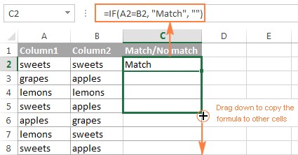
4.1.2. Comparing Two Cells for Equality

To compare two cells (e.g., A1 and B1) for equality, use the following formula:

=IF(A1=B1, "Match", "No Match")

This formula checks if the value in cell A1 is equal to the value in cell B1. If they match, it returns “Match”; otherwise, it returns “No Match”. This simple comparison is essential for verifying data integrity.

4.1.3. Comparing Two Cells for Inequality

To check if two cells are different, use the NOT operator in combination with the IF function, or use the <> operator directly. Here are both ways:

=IF(NOT(A1=B1), "Different", "Same")

Or, more concisely:

=IF(A1<>B1, "Different", "Same")

These formulas return “Different” if the values in A1 and B1 are not the same, and “Same” if they are identical. Using the inequality check is useful for quickly identifying discrepancies in your data.

4.1.4. Comparing Numbers and Dates

The IF function works equally well with numbers and dates. For example:

=IF(A1>B1, "A1 is greater", "B1 is greater or equal")

This formula checks if the value in A1 is greater than the value in B1. The result helps in sorting or filtering data based on numerical or chronological order.

4.1.5. Comparing Text Values (Case-Insensitive)

Excel’s default comparison is case-insensitive. This means it treats “Apple” and “apple” as the same.

=IF(A1=B1, "Match", "No Match")

This formula will return “Match” even if the case is different. For situations requiring case-sensitive comparisons, see the next section.

4.2. The EXACT Function: For Case-Sensitive Comparisons

When case sensitivity matters, the EXACT function ensures that the comparison is precise, distinguishing between uppercase and lowercase letters.

4.2.1. Syntax of the EXACT Function

The syntax for the EXACT function is straightforward:

=EXACT(text1, text2)

text1: The first text string.
text2: The second text string.

The function returns TRUE if the strings are identical (including case) and FALSE otherwise.

4.2.2. Implementing Case-Sensitive Comparison with IF and EXACT

Combine the EXACT function with the IF function to get a user-friendly result:

=IF(EXACT(A1, B1), "Exact Match", "Not an Exact Match")

This formula checks if the text in cell A1 is exactly the same as the text in cell B1, including case. It returns “Exact Match” if they are identical and “Not an Exact Match” if there’s any difference in case or content.

4.2.3. Example Use Case: Password Verification

A practical use case is verifying passwords. If you have a stored password in one cell and a user-entered password in another, use the EXACT function to ensure they match exactly. This ensures that security is maintained.

4.3. Combining Multiple Conditions with AND and OR

Sometimes, a single condition isn’t enough. The AND and OR functions allow you to combine multiple conditions to perform more complex comparisons.

4.3.1. Using the AND Function

The AND function checks if all conditions are true. Its syntax is:

=AND(condition1, condition2, ...)

condition1, condition2, ...: The conditions to evaluate.

4.3.2. Comparing Multiple Criteria with AND

For example, to check if both A1 and B1 are greater than 10, use:

=IF(AND(A1>10, B1>10), "Both are greater than 10", "At least one is not greater than 10")

This formula returns “Both are greater than 10” only if both cells meet the criteria; otherwise, it indicates that at least one cell does not meet the condition.

4.3.3. Using the OR Function

The OR function checks if at least one condition is true. Its syntax is:

=OR(condition1, condition2, ...)

condition1, condition2, ...: The conditions to evaluate.

4.3.4. Comparing Multiple Criteria with OR

To check if either A1 or B1 is greater than 10, use:

=IF(OR(A1>10, B1>10), "At least one is greater than 10", "Neither is greater than 10")

This formula returns “At least one is greater than 10” if either cell meets the condition, and “Neither is greater than 10” only if both cells are less than or equal to 10.

4.3.5. Combining AND and OR for Complex Logic

You can nest AND and OR functions to create complex logical tests. For example, check if A1 is greater than 10 and either B1 or C1 is greater than 5:

=IF(AND(A1>10, OR(B1>5, C1>5)), "Condition met", "Condition not met")

This formula offers a powerful way to implement intricate comparison logic.

5. Conditional Formatting for Visual Comparison

Conditional formatting in Excel provides a way to automatically apply formatting to cells based on specified criteria. This is particularly useful for visually highlighting differences or matches between cells.

5.1. Highlighting Differences

To highlight cells that differ from each other, follow these steps:

Select the cell (or range of cells) you want to format.
Go to Home > Conditional Formatting > New Rule.
Choose Use a formula to determine which cells to format.
Enter the formula =$A1<>$B1 (assuming you’re comparing column A to column B).
Click Format and choose a fill color or other formatting options.
Click OK to apply the rule.

This will highlight all cells in the selected range where the value is different from the corresponding cell in column B.

5.2. Highlighting Matches

To highlight cells that match each other, follow a similar process:

Select the cell (or range of cells) you want to format.
Go to Home > Conditional Formatting > New Rule.
Choose Use a formula to determine which cells to format.
Enter the formula =$A1=$B1.
Click Format and choose a fill color.
Click OK to apply the rule.

Now, all matching cells will be highlighted, making them easy to spot.

5.3. Using Color Scales to Indicate Variance

Color scales can visually represent the degree of difference between cells. To apply a color scale:

Select the range of cells you want to format.
Go to Home > Conditional Formatting > Color Scales.
Choose a color scale that suits your needs. For example, a green-yellow-red scale can indicate low, medium, and high variance.

Excel will automatically apply the color scale based on the values in the selected cells.

5.4. Icon Sets for Categorical Comparisons

Icon sets are useful for categorizing differences into predefined groups. For example:

Select the range of cells.
Go to Home > Conditional Formatting > Icon Sets.
Choose an icon set, such as arrows or flags.
Adjust the icon set rules as needed under Manage Rules to define the thresholds for each icon.

This allows you to quickly see which cells fall into different categories based on their values.

5.5. Managing Conditional Formatting Rules

To edit or remove conditional formatting rules:

Select the range of cells with the formatting.
Go to Home > Conditional Formatting > Manage Rules.
Select the rule you want to modify or delete.
Click Edit Rule to change the formatting or formula, or click Delete Rule to remove it.

Managing rules ensures that your formatting remains accurate and relevant as your data changes.

6. Advanced Techniques for Complex Comparisons

6.1. Comparing Entire Rows Based on Criteria

Sometimes, you need to compare entire rows based on criteria in specific columns. For example, highlight rows where the “Status” column is “Pending” and the “Due Date” is in the past.

Select the entire data range.
Go to Home > Conditional Formatting > New Rule.
Choose Use a formula to determine which cells to format.
Enter a formula like =AND($C1="Pending", $D1<TODAY()) (assuming column C is “Status” and column D is “Due Date”).
Choose a formatting style and apply the rule.

This will highlight all rows meeting both conditions.

6.2. Using VBA for Custom Comparison Functions

For highly customized comparisons, VBA (Visual Basic for Applications) allows you to create custom functions. For example, a function that compares two cells and returns a specific message based on the type of difference:

Press Alt + F11 to open the VBA editor.
Insert a new module (Insert > Module).
Write a function like:

Function CompareCells(cell1 As Range, cell2 As Range) As String
    If cell1.Value = cell2.Value Then
        CompareCells = "Cells are identical"
    ElseIf cell1.Value > cell2.Value Then
        CompareCells = "Cell 1 is greater"
    Else
        CompareCells = "Cell 2 is greater"
    End If
End Function

Use this function in your worksheet: =CompareCells(A1, B1).

VBA provides unparalleled flexibility for complex comparison scenarios.

6.3. Combining Formulas with Conditional Formatting

You can combine formulas with conditional formatting to create dynamic and insightful visualizations. For example, highlight cells that are within 10% of a target value:

Select the data range.
Go to Home > Conditional Formatting > New Rule.
Choose Use a formula to determine which cells to format.
Enter a formula like =AND(A1>=(TargetValue*0.9), A1<=(TargetValue*1.1)) where “TargetValue” is a cell containing the target value.
Apply the formatting.

This highlights cells that closely match the target, making it easy to identify values within an acceptable range.

7. Alternative Tools and Add-ins for Excel

While Excel’s built-in features are powerful, several add-ins and alternative tools can further enhance your comparison capabilities.

7.1. Kutools for Excel

Kutools is a comprehensive add-in that offers a variety of tools to simplify complex tasks in Excel, including advanced comparison features.

7.1.1. Features of Kutools

Compare Columns: Easily compare two columns and highlight differences or matches.
Compare Multiple Sheets: Compare data across multiple worksheets.
Advanced Select: Select cells based on complex criteria.

7.1.2. How to Use Kutools for Comparison

Install Kutools for Excel.
Select the columns you want to compare.
Use the Kutools tab to find the Compare Columns feature.
Specify your criteria and apply the comparison.

Kutools streamlines the comparison process with its intuitive interface.

7.2. ASAP Utilities

ASAP Utilities is another popular add-in that provides a range of functions to automate tasks and improve productivity in Excel.

7.2.1. Features of ASAP Utilities

Select Based on Content: Select cells based on specific content criteria.
Fill Missing Data: Automatically fill missing data based on patterns.
Advanced Sorting: Perform complex sorting operations.

7.2.2. How to Use ASAP Utilities for Comparison

Install ASAP Utilities.
Select the data range.
Use the ASAP Utilities menu to find the Select Based on Content feature.
Define your comparison criteria and apply the selection.

ASAP Utilities simplifies many data manipulation tasks, including comparison.

7.3. Beyond Compare

Beyond Compare is a dedicated file comparison tool that can also be used with Excel files. It offers advanced features for comparing files, folders, and data.

7.3.1. Features of Beyond Compare

Text Comparison: Compare text files, including CSV and Excel files.
Folder Comparison: Compare entire folder structures.
Data Comparison: Compare data within files.

7.3.2. How to Use Beyond Compare for Excel

Open your Excel files in Beyond Compare.
Use the text comparison feature to compare the data.
Review the differences and merge changes as needed.

Beyond Compare is ideal for users who need to compare complex data structures.

8. Best Practices for Comparing Cells in Excel

To ensure accurate and efficient comparisons, follow these best practices:

Data Consistency: Ensure your data is consistent in format and type.
Use Helper Columns: Use helper columns to simplify complex formulas.
Test Your Formulas: Always test your formulas to ensure they produce the correct results.
Document Your Steps: Document your comparison process for reproducibility.
Regularly Update Data: Keep your data up to date to avoid errors.

Following these practices will help you maintain data integrity and make informed decisions.

9. Real-World Examples and Use Cases

9.1. Financial Auditing

In financial auditing, comparing two cells is essential for verifying transactions and ensuring accuracy. For example, comparing entries in a general ledger with bank statements. Use the IF function to flag any discrepancies:

=IF(LedgerEntry<>BankStatementEntry, "Discrepancy", "Match")

9.2. Inventory Management

Comparing inventory counts from two different systems to identify discrepancies. Use conditional formatting to highlight differences:

Select the inventory count range.
Create a conditional formatting rule with the formula =$A1<>$B1.
Apply a red fill to highlight differences.

9.3. Academic Grading

Comparing grades from different assignments or exams to identify trends or inconsistencies. Use the AVERAGE function to calculate average scores and compare them:

=IF(AVERAGE(Exam1:Exam3)>AVERAGE(Assignment1:Assignment3), "Exams Higher", "Assignments Higher")

9.4. Sales Data Analysis

Comparing sales figures from different regions or time periods to identify top-performing areas or periods. Use color scales to visualize sales performance:

Select the sales data range.
Apply a color scale conditional formatting.
Use a green-yellow-red scale to indicate high, medium, and low sales.

9.5. Human Resources Management

Comparing employee data from different databases to ensure consistency and accuracy. Use the EXACT function to ensure case-sensitive matches for names and other text fields:

=IF(EXACT(Database1Name, Database2Name), "Match", "Discrepancy")

10. Troubleshooting Common Issues

10.1. Formulas Not Working

Check Syntax: Ensure your formula syntax is correct.
Cell References: Verify that your cell references are accurate.
Circular References: Avoid circular references in your formulas.

10.2. Conditional Formatting Not Applying

Rule Order: Check the order of your conditional formatting rules.
Formula Errors: Ensure your formulas are correct.
Overlapping Rules: Avoid overlapping rules that may conflict.

10.3. Incorrect Results

Data Types: Ensure your data types are consistent.
Hidden Characters: Check for hidden characters or spaces in your data.
Calculation Mode: Verify that your calculation mode is set to automatic.

11. COMPARE.EDU.VN: Your Partner in Data Comparison

Data comparison can be challenging, but with the right tools and techniques, it becomes manageable and insightful. COMPARE.EDU.VN is dedicated to providing comprehensive and objective comparisons to help you make informed decisions. Whether you are comparing products, services, or ideas, our platform offers detailed analyses and user reviews to guide you.

12. Call to Action: Explore More at COMPARE.EDU.VN

Ready to make data-driven decisions? Visit COMPARE.EDU.VN today to explore detailed comparisons and find the solutions that best fit your needs. Our platform offers objective analyses, user reviews, and side-by-side comparisons to help you make informed choices.

13. Contact Information

For more information or assistance, please contact us:

Address: 333 Comparison Plaza, Choice City, CA 90210, United States
WhatsApp: +1 (626) 555-9090
Website: COMPARE.EDU.VN

14. FAQs: Comparing Cells in Excel

14.1. How do I compare two cells in Excel for a simple match?

Use the formula =IF(A1=B1, "Match", "No Match") to check if cells A1 and B1 are the same.

14.2. How do I perform a case-sensitive comparison?

Use the formula =IF(EXACT(A1, B1), "Exact Match", "Not an Exact Match") to ensure the case matches.

14.3. Can I highlight differences between two cells automatically?

Yes, use conditional formatting with the formula =$A1<>$B1 to highlight cells that differ.

14.4. How can I compare two columns and highlight matches?

Use conditional formatting with the formula =$A1=$B1 to highlight cells in column A that match column B.

14.5. What is the best way to compare multiple columns for matches?

Use the COUNTIF function in combination with IF to check for matches across multiple columns. For example, =IF(COUNTIF($A1:$C1, $A1)=3, "Match", "No Match").

14.6. How can I compare two cells and return a custom message?

Use a nested IF function or a custom VBA function to return specific messages based on the comparison result.

14.7. Are there any add-ins that simplify cell comparison in Excel?

Yes, Kutools for Excel and ASAP Utilities are popular add-ins that offer advanced comparison features.

14.8. How do I compare two cells containing dates?

Use the same IF function as with numbers: =IF(A1>B1, "A1 is later", "B1 is later or equal").

14.9. Can I compare two cells based on multiple criteria?

Yes, use the AND and OR functions to combine multiple conditions in your comparison formula.

14.10. How can I troubleshoot formulas that are not working correctly?

Check your formula syntax, cell references, and data types, and ensure that your calculation mode is set to automatic.

By using these comprehensive methods and resources, you can effectively compare cells in Excel, highlight differences, and make informed decisions based on accurate data analysis. Let compare.edu.vn be your trusted partner in navigating the complexities of data comparison.

Formula Comparison