Comparing two columns in Excel can be a daunting task, especially when dealing with large datasets. But with the right techniques, you can streamline your data analysis and unlock valuable insights. At COMPARE.EDU.VN, we offer a comprehensive guide to help you master the art of comparing columns in Excel, using various methods from simple formulas to advanced conditional formatting. Learn how to efficiently identify matching, mismatching, unique, and duplicate values, enabling you to make informed decisions with confidence. Explore effective data comparison techniques and improve data accuracy.
1. Understanding the Importance of Column Comparison in Excel
Excel is a powerful tool for data storage, manipulation, and analysis. Its versatility makes it indispensable for data analysts who play a critical role in marketing, sales, and various other decision-making processes. Comparing two columns within an Excel spreadsheet or across different spreadsheets is often necessary to identify discrepancies, missing data, or to validate data integrity. Manually comparing these columns can be time-consuming and prone to error, especially when dealing with large datasets. This is where the techniques discussed in this guide become invaluable.
1.1. Why Compare Columns?
Column comparison is essential for several reasons:
- Data Validation: Ensuring the accuracy and consistency of data across different sources.
- Data Cleaning: Identifying and correcting errors, inconsistencies, and missing values.
- Data Analysis: Uncovering patterns, trends, and relationships within data.
- Decision Making: Providing reliable information for informed decision-making.
1.2. Scenarios Where Column Comparison is Useful
- Inventory Management: Comparing a list of available products with a list of sold products to identify what needs to be restocked.
- Customer Relationship Management (CRM): Comparing a list of customer email addresses with a list of unsubscribed addresses to ensure compliance with email marketing regulations.
- Financial Auditing: Comparing financial records from different departments to identify discrepancies.
- Research Analysis: Comparing survey responses from different groups to identify significant differences.
- Academic Research: Comparing different student results on excel.
2. Methods for Comparing Two Columns in Excel
There are various methods for comparing two columns in Excel, each with its own strengths and weaknesses. The best method for you will depend on the specific task and the size of your dataset. Here are some of the most common techniques:
- Using the Equals Operator (=)
- Using the IF Condition
- Using the EXACT() Function
- Using Conditional Formatting
- Using LOOKUP Functions
3. Comparing Columns with the Equals Operator (=)
The equals operator (=) is the simplest way to compare two columns in Excel on a row-by-row basis. This method is best suited for identifying exact matches between corresponding cells in the two columns.
3.1. How to Use the Equals Operator
- Select an empty column next to the columns you want to compare.
- In the first cell of the empty column (e.g., C2), enter the formula
=A2=B2, where A2 and B2 are the first cells in the columns you want to compare. - Press Enter. The formula will return
TRUEif the values in A2 and B2 are identical, andFALSEotherwise. - Drag the fill handle (the small square at the bottom-right corner of the cell) down to apply the formula to the rest of the rows in your data.
3.2. Interpreting the Results
- TRUE: Indicates that the values in the corresponding rows of the two columns are exactly the same.
- FALSE: Indicates that the values in the corresponding rows of the two columns are different.
3.3. Example
Let’s say you have two columns, “Product ID” (Column A) and “Database ID” (Column B), and you want to check if the IDs match in each row.
| Product ID (A) | Database ID (B) | Match? (C) |
|---|---|---|
| 12345 | 12345 | TRUE |
| 67890 | 67890 | TRUE |
| 13579 | 24680 | FALSE |
| 24680 | 24680 | TRUE |
In cell C2, you would enter the formula =A2=B2 and drag it down to C5. The “Match?” column would then display TRUE for rows where the IDs match and FALSE where they don’t.
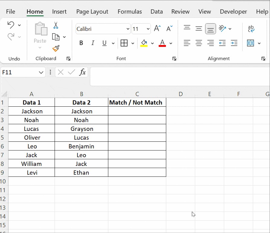
4. Comparing Columns with the IF Condition
The IF condition allows you to compare two columns and return custom messages based on whether the values match or mismatch. This method provides more flexibility than the equals operator, as you can define your own output messages.
4.1. How to Use the IF Condition
- Select an empty column next to the columns you want to compare.
- In the first cell of the empty column (e.g., C2), enter the formula
=IF(A2=B2,"Match","Mismatch"), where A2 and B2 are the first cells in the columns you want to compare. - Press Enter. The formula will return “Match” if the values in A2 and B2 are identical, and “Mismatch” otherwise.
- Drag the fill handle down to apply the formula to the rest of the rows in your data.
4.2. Customizing the Output Messages
You can customize the output messages in the IF formula to suit your specific needs. For example, you could use “Duplicate” and “Unique” instead of “Match” and “Mismatch”.
4.3. Example
Using the same “Product ID” and “Database ID” example as before, you can use the IF condition to display “Match” or “Not a Match” in the “Status” column:
| Product ID (A) | Database ID (B) | Status (C) |
|---|---|---|
| 12345 | 12345 | Match |
| 67890 | 67890 | Match |
| 13579 | 24680 | Not a Match |
| 24680 | 24680 | Match |
The formula in cell C2 would be =IF(A2=B2,"Match","Not a Match").
5. Comparing Columns with the EXACT() Function
The EXACT() function is similar to the equals operator and the IF condition, but it is case-sensitive. This means that it will only return TRUE or “Match” if the values in the two cells are identical, including their case. This function is particularly useful when comparing text strings where case sensitivity matters.
5.1. How to Use the EXACT() Function
- Select an empty column next to the columns you want to compare.
- In the first cell of the empty column (e.g., C2), enter the formula
=IF(EXACT(A2,B2),"Match","Mismatch"), where A2 and B2 are the first cells in the columns you want to compare. - Press Enter. The formula will return “Match” if the values in A2 and B2 are exactly the same (including case), and “Mismatch” otherwise.
- Drag the fill handle down to apply the formula to the rest of the rows in your data.
5.2. Example
Consider two columns, “Name” (Column A) and “Name (Corrected)” (Column B), where you need to ensure that the names are identical, including capitalization:
| Name (A) | Name (Corrected) (B) | Status (C) |
|---|---|---|
| John Doe | John Doe | Match |
| Jane Smith | jane Smith | Mismatch |
| Peter Jones | Peter Jones | Match |
| Mary Brown | Mary Brown | Match |
The formula in cell C2 would be =IF(EXACT(A2,B2),"Match","Mismatch"). Notice that “Jane Smith” and “jane Smith” are considered a mismatch due to the case difference.
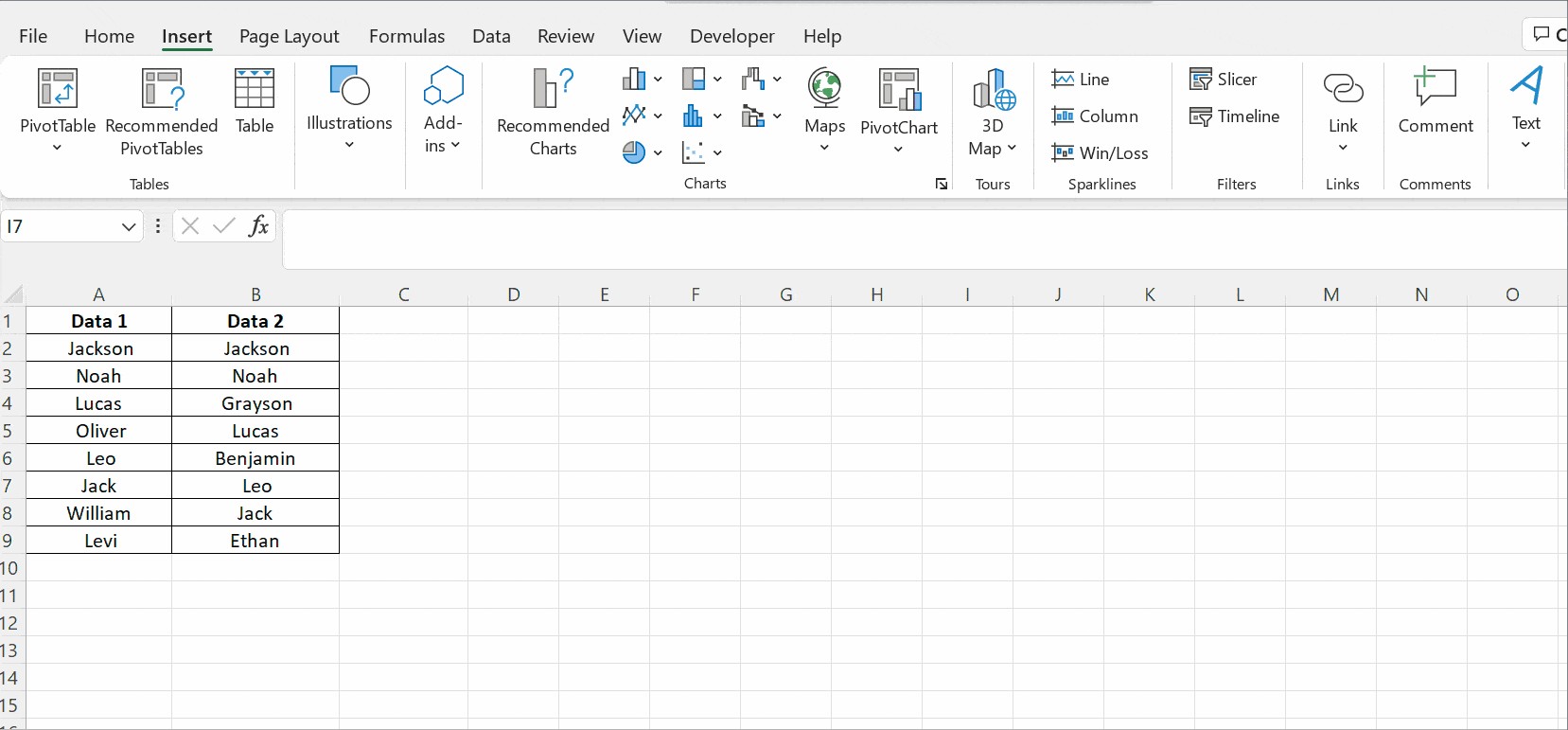
6. Comparing Columns with Conditional Formatting
Conditional formatting allows you to highlight cells that meet specific criteria, making it easy to visually identify matching, mismatching, unique, or duplicate values. This method is particularly useful for large datasets where you need to quickly identify patterns.
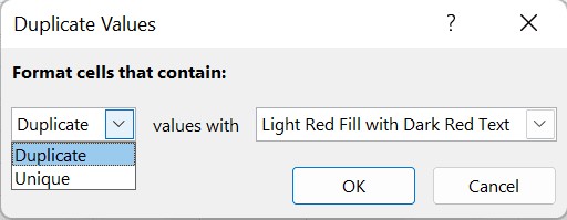
6.1. Highlighting Duplicate Values
- Select the columns you want to compare.
- Go to Home > Conditional Formatting > Highlight Cells Rules > Duplicate Values.
- Choose the formatting you want to apply to duplicate values (e.g., fill with red).
- Click OK. Excel will highlight all the duplicate values in the selected columns.
6.2. Highlighting Unique Values
- Select the columns you want to compare.
- Go to Home > Conditional Formatting > Highlight Cells Rules > Duplicate Values.
- In the dialog box, choose “Unique” from the dropdown menu.
- Choose the formatting you want to apply to unique values (e.g., fill with green).
- Click OK. Excel will highlight all the unique values in the selected columns.
6.3. Example
Suppose you have two columns, “Customer List 1” (Column A) and “Customer List 2” (Column B), and you want to identify customers who appear in both lists (duplicates) and those who appear only in one list (unique):
| Customer List 1 (A) | Customer List 2 (B) |
|---|---|
| John Doe | Jane Smith |
| Jane Smith | Peter Jones |
| Peter Jones | John Doe |
| Mary Brown | David Lee |
Using conditional formatting, you can highlight the duplicate names (John Doe, Jane Smith, Peter Jones) in one color and the unique names (Mary Brown, David Lee) in another color.
7. Comparing Columns with LOOKUP Functions
LOOKUP functions, such as VLOOKUP, HLOOKUP, and XLOOKUP, allow you to search for a specific value in one column and return a corresponding value from another column. These functions are particularly useful for comparing two columns and identifying values that exist in one column but not in the other.
7.1. Using VLOOKUP to Find Missing Values
VLOOKUP (Vertical LOOKUP) searches for a value in the first column of a range and returns a value from a specified column in the same row.
- Select an empty column next to the column you want to search in (e.g., Column C next to Column A).
- In the first cell of the empty column (e.g., C2), enter the formula
=VLOOKUP(A2,B:B,1,FALSE), where A2 is the first cell in the column you want to search for, B:B is the column you want to search in, 1 is the column number to return (in this case, it’s the same column you’re searching in), and FALSE specifies an exact match. - Press Enter. If the value in A2 is found in Column B, the formula will return the value. If the value is not found, the formula will return
#N/A. - Drag the fill handle down to apply the formula to the rest of the rows in your data.
7.2. Interpreting the Results
- Value: Indicates that the value in Column A exists in Column B.
- #N/A: Indicates that the value in Column A does not exist in Column B.
7.3. Example
Suppose you have a list of registered users (Column A) and a list of active users (Column B), and you want to identify which registered users are not active:
| Registered Users (A) | Active Users (B) | Status (C) |
|---|---|---|
| John Doe | John Doe | John Doe |
| Jane Smith | Peter Jones | #N/A |
| Peter Jones | Mary Brown | Peter Jones |
| Mary Brown | Mary Brown | |
| David Lee | #N/A |
The formula in cell C2 would be =VLOOKUP(A2,B:B,1,FALSE). The #N/A values in Column C indicate that Jane Smith and David Lee are registered but not active.
7.4. Using the ISNA Function with VLOOKUP for Clarity
To make the results more user-friendly, you can combine the VLOOKUP function with the ISNA function. The ISNA function checks if a value is #N/A and returns TRUE if it is, and FALSE otherwise.
- Use the same VLOOKUP formula as before:
=VLOOKUP(A2,B:B,1,FALSE) - Wrap this formula inside the ISNA function:
=ISNA(VLOOKUP(A2,B:B,1,FALSE)) - Now, the result will be TRUE if the value is not found (previously #N/A) and FALSE if the value is found.
- To display custom messages, use the IF condition with the ISNA function:
=IF(ISNA(VLOOKUP(A2,B:B,1,FALSE)),"Not Active","Active")
The updated example would look like this:
| Registered Users (A) | Active Users (B) | Status (C) |
|---|---|---|
| John Doe | John Doe | Active |
| Jane Smith | Peter Jones | Not Active |
| Peter Jones | Mary Brown | Active |
| Mary Brown | Active | |
| David Lee | Not Active |
The formula in cell C2 would be =IF(ISNA(VLOOKUP(A2,B:B,1,FALSE)),"Not Active","Active"). This provides a clearer indication of the status of each user.
8. Advanced Techniques for Comparing Columns
Beyond the basic methods, there are more advanced techniques that can be used for more complex comparison scenarios. These include:
8.1. Using Array Formulas
Array formulas allow you to perform calculations on multiple values at once. They can be used to compare two columns and return an array of results, which can then be analyzed using other functions.
8.1.1. Example: Counting Matches
To count the number of matching values between two columns, you can use the following array formula:
=SUM(IF(A1:A10=B1:B10,1,0))
Note: To enter an array formula, you must press Ctrl+Shift+Enter instead of just Enter.
This formula compares the values in A1:A10 with the values in B1:B10. If the values in the corresponding rows are equal, the formula returns 1; otherwise, it returns 0. The SUM function then adds up all the 1s to give you the total number of matches.
8.2. Using Power Query
Power Query (also known as Get & Transform Data) is a powerful data transformation and analysis tool built into Excel. It can be used to compare two columns from different tables and identify matching, mismatching, unique, or duplicate values.
8.2.1. Steps to Compare Columns Using Power Query
- Load the data into Power Query.
- Merge the queries based on the columns you want to compare.
- Expand the columns from the merged query.
- Filter the rows based on the comparison results.
8.3. Using VBA (Visual Basic for Applications)
VBA is a programming language that can be used to automate tasks in Excel. It can be used to compare two columns and perform complex operations based on the comparison results.
8.3.1. Example: Highlighting Mismatches in Different Colors
The following VBA code compares two columns and highlights the mismatches in different colors:
Sub CompareColumns()
    Dim LastRow As Long
    Dim i As Long

    'Find the last row with data in column A
    LastRow = Cells(Rows.Count, "A").End(xlUp).Row

    'Loop through each row
    For i = 2 To LastRow 'Assuming data starts from row 2
        'Compare the values in column A and column B
        If Cells(i, "A").Value <> Cells(i, "B").Value Then
            'Highlight the mismatching cells
            Cells(i, "A").Interior.Color = RGB(255, 0, 0) 'Red
            Cells(i, "B").Interior.Color = RGB(0, 0, 255) 'Blue
        End If
    Next i
End Sub
This code loops through each row of the specified columns, compares the values, and highlights the mismatches in red and blue.
9. Best Practices for Comparing Columns in Excel
To ensure accurate and efficient column comparison, follow these best practices:
- Prepare Your Data: Before comparing columns, make sure your data is clean and consistent. Remove any unnecessary spaces, special characters, or formatting that could affect the comparison results.
- Choose the Right Method: Select the comparison method that is most appropriate for your specific task. Consider the size of your dataset, the type of data you are comparing, and the level of detail you need.
- Use Absolute References: When using formulas, use absolute references ($) to lock the cell references. This will prevent errors when you drag the formulas down to apply them to the rest of your data.
- Test Your Formulas: Before applying formulas to your entire dataset, test them on a small sample to ensure that they are working correctly.
- Document Your Steps: Keep a record of the steps you took to compare the columns, including the formulas you used and the results you obtained. This will help you to reproduce the results later and to troubleshoot any problems that may arise.
10. Common Mistakes to Avoid
- Ignoring Case Sensitivity: Be aware of whether your comparison method is case-sensitive or not. If you need to compare text strings in a case-sensitive manner, use the EXACT() function.
- Comparing Different Data Types: Make sure you are comparing data of the same type. For example, don’t compare text strings with numbers.
- Overlooking Hidden Characters: Hidden characters, such as spaces or non-printing characters, can affect the comparison results. Use the TRIM() function to remove any leading or trailing spaces.
- Using Incorrect Cell References: Double-check your cell references to make sure you are comparing the correct columns and rows.
- Not Testing Your Formulas: Always test your formulas on a small sample before applying them to your entire dataset.
11. Optimizing Excel Performance for Large Datasets
When working with large datasets, Excel can become slow and unresponsive. To optimize performance, try these tips:
- Use Formulas Efficiently: Avoid using volatile functions, such as NOW() and RAND(), which recalculate every time the spreadsheet changes.
- Disable Automatic Calculations: Set the calculation mode to manual and recalculate the spreadsheet only when necessary.
- Use Named Ranges: Use named ranges to make your formulas more readable and efficient.
- Filter Data: Use filters to display only the data you need to see.
- Use Excel Tables: Excel tables are more efficient than regular ranges.
- Close Unnecessary Workbooks: Close any workbooks that you are not currently using.
- Increase Memory Allocation: Increase the amount of memory allocated to Excel.
- Upgrade Your Hardware: If you are still experiencing performance problems, consider upgrading your hardware.
12. Frequently Asked Questions (FAQ)
1. How do I compare two columns in Excel and highlight the differences?
You can use conditional formatting to highlight the differences between two columns. Select the columns, go to Home > Conditional Formatting > New Rule > Use a formula to determine which cells to format. Enter a formula like =A1<>B1 and choose the formatting you want to apply to the different cells.
2. How do I compare two columns in Excel for partial matches?
You can use the SEARCH() or FIND() function to compare two columns for partial matches. These functions return the starting position of one text string within another text string.
3. How do I compare two columns in Excel and return a value from another column?
You can use the VLOOKUP, HLOOKUP, or INDEX-MATCH functions to compare two columns and return a value from another column.
4. How do I compare two columns in Excel and count the number of matches?
You can use the COUNTIF() function or an array formula to count the number of matches between two columns.
5. How do I compare two columns in Excel and identify the unique values?
You can use conditional formatting to highlight the unique values in two columns.
6. How do I compare two columns in Excel and find the missing values?
You can use the VLOOKUP function or Power Query to find the missing values between two columns.
7. How do I compare two columns in Excel and ignore case?
You can use the UPPER() or LOWER() function to convert the text strings to the same case before comparing them.
8. How do I compare two columns in Excel and remove duplicates?
You can use the Remove Duplicates feature in Excel to remove duplicate values from two columns.
9. How do I compare two columns in Excel and sort them?
You can use the SORT function to sort the columns before comparing them.
10. How do I compare two columns in Excel and merge them?
You can use Power Query to merge two columns based on the comparison results.
13. Conclusion: Mastering Column Comparison in Excel
Comparing two columns in Excel is a fundamental skill for data analysts, enabling them to validate data, identify discrepancies, and extract valuable insights. This comprehensive guide has provided you with a range of techniques, from simple formulas to advanced conditional formatting and LOOKUP functions. By understanding and applying these methods, you can streamline your data analysis workflow and make informed decisions with confidence.
Remember to choose the right method for your specific task, prepare your data carefully, and test your formulas before applying them to your entire dataset. By following these best practices, you can avoid common mistakes and optimize Excel performance for large datasets.
At COMPARE.EDU.VN, we are committed to providing you with the knowledge and resources you need to excel in data analysis. This guide is just one example of the many valuable resources we offer. Visit our website at COMPARE.EDU.VN to explore more articles, tutorials, and tools that can help you master Excel and other data analysis skills.
14. Ready to Take Your Excel Skills to the Next Level?
Don’t let data discrepancies hold you back. Visit COMPARE.EDU.VN today to discover more comprehensive guides, tutorials, and resources that will empower you to master Excel and unlock the full potential of your data.
Our platform offers:
- In-depth comparisons of various Excel techniques
- Step-by-step tutorials with clear examples
- Expert advice from experienced data analysts
- A supportive community of Excel users
Stop struggling with data comparison and start making informed decisions with confidence. Visit COMPARE.EDU.VN now!
For more information, contact us at:
- Address: 333 Comparison Plaza, Choice City, CA 90210, United States
- WhatsApp: +1 (626) 555-9090
- Website: COMPARE.EDU.VN
Let compare.edu.vn be your trusted partner in mastering Excel and achieving your data analysis goals.