Comparing data across multiple cells is a common task in Excel. This tutorial provides a step-by-step guide on How To Compare Three Cells In Excel using a simple formula and conditional formatting. This method allows you to quickly identify matches and discrepancies within your data.
Using the IF and AND Functions for Comparison
The core of this comparison technique lies in combining the IF and AND functions. The AND function checks if multiple conditions are true. The IF function then returns a specified value if the AND condition is met and another value if it’s not.
Here’s the formula:
=IF(AND(B2=C2,C2=D2),"Equal","Not Equal")Let’s break down this formula:
IF(condition, value_if_true, value_if_false): This function evaluates a condition. If the condition is true, it returnsvalue_if_true; otherwise, it returnsvalue_if_false.AND(logical1, [logical2], ...): This function returnsTRUEif all of its arguments are true; otherwise, it returnsFALSE.B2=C2, C2=D2: These are the comparison conditions. The formula checks if the value in cellB2is equal to the value inC2, and if the value inC2is equal to the value inD2.
In essence, the formula checks if the values in cells B2, C2, and D2 are all equal. If they are, it returns “Equal”; otherwise, it returns “Not Equal”.
Practical Example: Comparing Basketball Scores
Imagine you have a dataset of the highest scorers for different basketball teams across three games:
To compare the highest scorer for each team across all three games, you would enter the formula =IF(AND(B2=C2,C2=D2),"Equal","Not Equal") in cell E2:
The formula returns “Not Equal” for the first row because the names don’t match across all three columns. You can then drag this formula down to apply it to the remaining rows:
Highlighting Matches with Conditional Formatting
To visually highlight rows where all three cells are equal, you can use conditional formatting:
- Select the cell range containing the results (e.g.,
E2:E11). - Go to Home > Conditional Formatting > Highlight Cells Rules > Equal To.
- Enter “Equal” in the input box and choose a formatting style (e.g., green fill).
This will highlight the rows with matching values:
This combination of the IF and AND functions with conditional formatting provides a powerful way to compare three cells in Excel and easily identify matching data. This technique can be adapted to various scenarios for efficient data analysis.